What is Logistic Regression?
Logistic Regression is a machine learning technique that is used to model the probability of an event or class having a binary outcome. Logistic Regression is a technique mostly used in industry to model for binary classification problems. Binary outcome means the dependent variable can have only two possible values, viz, Yes / No (1 or 0)
Applications of Logistic Regression Model:
Marketing – Whether the customer will respond to the offer or not
Risk in Lending Business – Whether the customer being given loan will repay or not
HR – Whether an employee will attrite or not
Machine – When an appliance will breakdown or not
When the above business problems are converted to mathematical form, the occurrence of an event is typically labeled as 1, and non-occurrence is labeled as 0.
Logistic vs Linear Regression?
Logistic regression is used when the dependent variable is binary (1 / 0)
Linear regression is used when the dependent variable is continuous ( – inf. to + inf.)
In a binary classification problem, the value of the dependent variable is bounded between 0 & 1 as such Linear regression cannot be used. To restrict the predicted value of the regression model between 0 and 1, a generalized form of linear regression called logistic regression is used.
The logistic regression equation format is shown below:
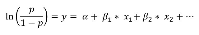
Where:
p is the probability of event occurrence
1-p is the probability of event non-occurrence
Understanding logistic regression concept with data
We will consider a hypothetical data to understand the concept of logistic regression as shown in the table below.
Note: The entire data file named LR_DF.csv can be downloaded from our resources section.
| Cust_ID | Target | Age |
| C1 | 0 | 30 |
| C2 | 0 | 43 |
| C3 | 0 | 53 |
| C4 | 0 | 45 |
| C5 | 0 | 37 |
| C6 | 0 | 41 |
| C7 | 1 | 46 |
| C8 | 1 | 33 |
| .. | .. | .. |
| C20000 | 1 | 43 |
Independent Variable – Age is an independent variable in the above data.
Dependent Variable – Target is our binary clas, dependent variable where 1 is a responder to the marketing offer and 0 is non-responder class.
Where is the probability?
The value in the Target column for each row is 0 or 1.
Just imagine, you aggregate the data by Age and compute the percentage of customers responding in each age group, i.e. response probability. The sample table structure to explain the probability calculation is shown below.
| Age | Target = 0 | Target = 1 | Total | Resp. Probability |
| 21 | 207 | 5 | 212 | 0.024 |
| 22 | 241 | 7 | 248 | 0.028 |
| 23 | 375 | 9 | 384 | 0.023 |
| 24 | 375 | 21 | 396 | 0.053 |
| 25 | 531 | 13 | 544 | 0.024 |
| 26 | 591 | 21 | 612 | 0.034 |
| 27 | 600 | 12 | 612 | 0.020 |
| 28 | 718 | 30 | 748 | 0.040 |
The logistic regression is designed to model the relationship between the probability and the independent variable.
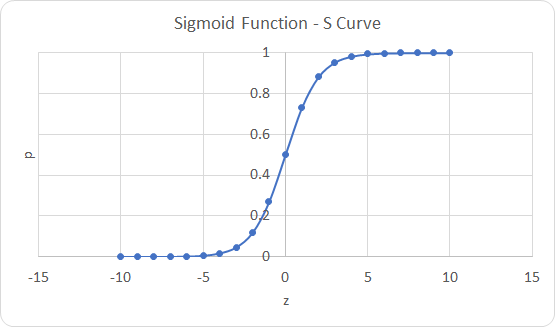
Logistic Function (Sigmoid Function)
Let us know see the mathematical steps to express the below equation in probability form.
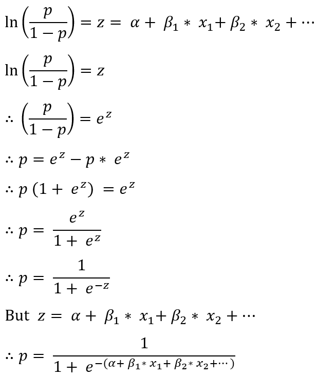
The function p= 1/(1+ e^(-z) ) is called the Logistic Function.
S-Curve (Sigmoid Function)
If we make a plot of p vs z based on logistic function, p= 1/(1+ e^(-z) ), we will get an S-curve as shown in the plot. Because of the s-curve, the logistic function is also a sigmoid function.
| z | p | z | p | |
| 0 | 0.500000 | 0 | 0.500000 | |
| -1 | 0.268941 | 1 | 0.731059 | |
| -2 | 0.119203 | 2 | 0.880797 | |
| -3 | 0.047426 | 3 | 0.952574 | |
| -4 | 0.017986 | 4 | 0.982014 | |
| -5 | 0.006693 | 5 | 0.993307 | |
| -6 | 0.002473 | 6 | 0.997527 | |
| -7 | 0.000911 | 7 | 0.999089 | |
| -8 | 0.000335 | 8 | 0.999665 | |
| -9 | 0.000123 | 9 | 0.999877 | |
| -10 | 0.000045 | 10 | 0.999955 |

The sigmoid function, s-curve has two horizontal asymptotes. Both ends of the s curve is an asymptote.
What is an asymptote?
Logistic Regression Blog Series Links
Business Objective Statement: MyBank wishes to develop a Direct Marketing Channel to sell their loan products to existing deposit account customers. The bank executed a pilot campaign to cross-sell personal loans to its existing customers. A random base of 20000 customers was targeted with an attractive personal loan offer and processing fee waiver. The data of the customers who were targeted and their response to the marketing offer has been provided. The data is in the file (LR_DF.csv) and it can be downloaded from our resources section.
We will use the above business case to explain the concepts of Logistic Regression along with R and Python code in this blog series. The links to various modules of the blog series are given below:
| Sr. No. | Logistic Regression blog-series | R | Python |
| 1. | Introduction to Logistic Regression | ||
| 2. | Hypothesis Development | Link | |
| 3. | Single Variable Logistic Regression Model Development & Model Summary Interpretation | Link | |
| 4. | Training and Testing | Link | |
| 5. | Splitting Data in Dev – Validation – Holdout Sample | Link | |
| 6A. | Information Value Concept | Link | |
| 7. | Outlier Treatment | Link | |
| 8. | Missing Value Imputation | Importance of Missing Value Imputation | |
| 9. | Visualization and Pattern Detection | Visualization using Double Axis Charts and Log-Odds Plot | |
| 10. | Weight of Evidence | WoE | |
| 11. | Model Development | Multiple Logistic Regression | |
| 12. | Model Performance Measurement | Rank Order, KS, Lift Chart Classification Accuracy, AUC-ROC Concordance, Gini, Goodness of Fit |
|
| 13. | Model Validation | Link | Link |
| 14. | Hold-out Testing | Link | Link |
| 15. | Model Implementation & Deployment Strategy | Link | Link |
Recent Comments