In this blog, we will see how to impute a categorical variable using the KNN technique in Python.
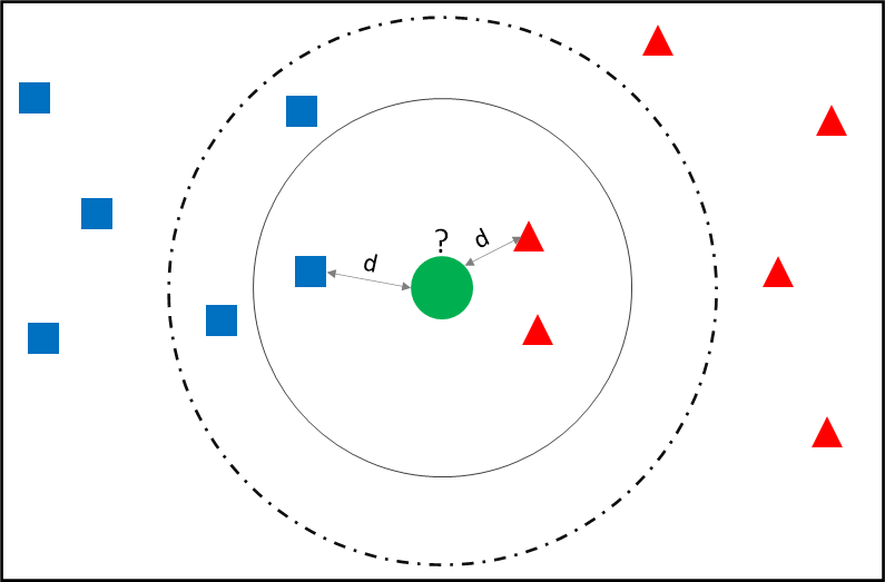
Pre-read: K Nearest Neighbour Machine Learning Algorithm
Missing Value Imputation of Categorical Variable (with Python code)
Dataset
We will continue with the development sample as created in the training and testing step. The categorical variable, Occupation, has missing values in it. Let us check the missing.
Check for missingness
count_row = dev.shape[0]
count_occupation = dev["Occupation"].count()

print("No. of rows =",  count_row)
print("Occupation count =",  count_occupation)
print("No. of rows with missing occupation =", (count_row - count_occupation))
Occupation count = 7706
No. of rows with missing occupation = 2294
Frequency Distribution
freq_table = dev["Occupation"].value_counts().to_frame()
freq_table.reset_index(inplace=True) # reset index
freq_table.columns = [ "Occupation" , "Count"] # rename columns
freq_table["Pct_Obs"] = round(freq_table['Count'] / sum(freq_table['Count']),2)
freq_table
| Occupation | Count | Pct_Obs | |
|---|---|---|---|
| 0 | SAL | 2987 | 0.39 |
| 1 | PROF | 2734 | 0.35 |
| 2 | SELF-EMP | 1643 | 0.21 |
| 3 | SENP | 342 | 0.04 |
Imputation using KNN with Python code
# Select Age, Balance, No_OF_CR_TXNS and Occupation variables
# selecting only non missing records
dev_knn = dev.iloc[:, [2, 4, 6, 5]].dropna()
X_train = dev_knn.iloc[:, 0:3]
y_train = dev_knn.iloc[:, 3]
## Creating the K Nearest Neighbour Classifier Object
## I have not normalized the variables as such using KD Tree algorithm

from sklearn.neighbors import KNeighborsClassifier
knn_model = KNeighborsClassifier(n_neighbors = 21, weights = 'uniform',
metric = 'euclidean', algorithm = 'kd_tree')
knn_model.fit(X_train, y_train)
## Imputing the values for missing occupation
def impute_missing_occ (row):
    if pd.isnull(row['Occupation']) :
        return knn_model.predict(
            row[["Age","Balance","No_OF_CR_TXNS"]].values.reshape((-1, 3)))
    else:
        return row[['Occupation']]
dev["Occ_KNN_Imputed"] = dev.apply(impute_missing_occ,axis=1)
Compare the distribution
Compare the frequency distribution of imputed occupation with the original distribution. There mustn’t be much change in the distribution because of the imputation. If there is a significant change in then probably the imputation logic is not correct.
freq_table = dev["Occ_KNN_Imputed"].value_counts().to_frame()
freq_table.reset_index(inplace=True) # reset index
freq_table.columns = [ "Occ_KNN_Imputed" , "Count"] # rename columns
freq_table["Pct_Obs"] = round(freq_table['Count'] / sum(freq_table['Count']),2)
freq_table
| Occupation | Count | Pct_Obs | |
|---|---|---|---|
| 0 | SAL | 3979 | 0.40 |
| 1 | PROF | 3780 | 0.38 |
| 2 | SELF-EMP | 1875 | 0.19 |
| 3 | SENP | 366 | 0.04 |
Conclusion
As there is not much difference in frequency distribution before and after imputation, we may assume the imputation has happened correctly.
<<< previous blog | next blog >>>
Logistic Regression blog series home
Recent Comments