So far in our previous blogs, we have learned Rank Order, K-S, Gains table, Lift, Classification Accuracy, Precision, Recall, Sensitivity-Specificity, AUC-ROC Curve. In this blog, we will learn three more important model performance measures – Concordance – Discordance, Gini Coefficient, and Goodness of Fit.
Concordance – Discordance
A binary classifier model is built to predict the likelihood of a record belonging to 1 / 0, where 1 is used to represent the occurrence of the phenomenon of interest, and 0 for non-occurrence. It is expected that the model will assign a relatively higher probability to one’s and lower probability to zero’s. Assume, we take a random pair of 1 & 0 from data and compare their probabilities as assigned by the predictive model. If the probability assigned to 1 is higher than the probability assigned to 0 in the pair then, the pair is said to be Concordant. If the probabilities assigned to 1 & 0 in the pair is equal then, it is a Tied pair. If the probability of 0 is more than 1 then, the pair is Discordant pair.
Concordance Calculations
We will understand the concordance calculations using the sample data shown below.
| ID | Target | Probability |
| 1 | 0 | 0.056 |
| 2 | 0 | 0.134 |
| 3 | 0 | 0.156 |
| 4 | 1 | 0.200 |
| 5 | 0 | 0.200 |
| 6 | 0 | 0.273 |
| 7 | 1 | 0.250 |
| 8 | 1 | 0.512 |
| 9 | 0 | 0.135 |
| 10 | 0 | 0.089 |
In the above data:
- Three records (ID – 4, 7, and 8) have the Target value as 1
- Seven records have Target value 0
From data, we can create 3 * 7 = 21 pairs of 1, and 0. One set of these pairs and their classification as Concordant, Discordant, or Tied is explained below.
| Pair (1, 0) |
Probabilities (1, 0) |
C | D | T | Explanation |
| 4,1 | 0.200, 0.056 | C | In the pair, the probability of 1 is more than that of 0 as such the pair is Concordant |
| 4,2 | 0.200, 0.134 | C | |
| 4,3 | 0.200, 0.156 | C | |
| 4,5 | 0.200, 0.200 | T | The probability of 1 is equal to that of 0 as such the pair is Tied |
| 4,6 | 0.200, 0.273 | D | The probability of 1 is less than that of 0 as such the pair is Discordant |
| 4,9 | 0.200, 0.135 | C | |
| 4,10 | 0.200, 0.089 | C |
Likewise, we have to create the other pairs of 1 & 0. The total number of pairs formed from the above data is 21. Out of 21 pairs, 18 are Concordant, 2 Discordant, and 1 Tied. The Concordance is 85.7% (=18/21).
Note: 1) A good classification model should have concordance above 80%.
Gini Coefficient
Gini Coefficient in Economics
The Gini Coefficient is an index to measure inequality. It is a measure first developed to measure how unequal is the distribution of wealth in the society. The higher the Gini, the more the inequality.
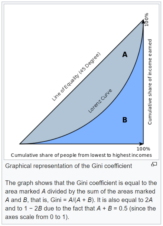 [ Source: Wikipedia] The Gini coefficient is usually defined mathematically based on the Lorenz curve, which plots the proportion of the total income of the population (y-axis) that is cumulatively earned by the bottom x of the population (see diagram). The line at 45 degrees thus represents perfect equality of incomes. The Gini coefficient can then be thought of as the ratio of the area that lies between the line of equality and the Lorenz curve (marked A in the diagram) over the total area under the line of equality (marked A and B in the diagram); i.e., G = A/(A + B).
Gini Coefficient in Binary Classifier Model
In machine learning, the Gini Coefficient is used to evaluate the performance of Binary Classifier Models. The value of the Gini Coefficient can be between 0 to 1. The higher the Gini coefficient, the better is the model.
In Economics, the income of population from lowest to highest is plotted on the X-axis, whereas, in the Binary Classifier Model we go through the model probability predictions from lowest to highest on X-axis. On Y-axis, instead of summing up the wealth (as in Economics), we sum up the Actuals Values of the predictions to get the Lorenz Curve of the model.
Mathematically we can easily derive Gini from AUC using the formula: Gini = 2 * AUC – 1
Note: Gini above 60% is a good model.
Hosmer-Lemeshow Goodness of Fit test (HL-GoF test)
HL-GOF test is used to see how good the model fits the data. It is very similar to the CHI-SQ Goodness of Fit test. The test hypothesis is:
Null Hypothesis: There is no significant difference between the actual and the predicted values, i.e. the model fits the data well.
Alternate Hypothesis: There is a significant difference between the actual and the predicted values, i.e. the model is not fits the data well.
The HL-GoF test is done by splitting the data into g groups (usually g = 10) based on the predicted probabilities. For each group, you get the count of the actual number of responders (Target = 1) and the number of non-responders (Target = 0). The p-value is computed using the Chi-Sq test with a g-2 degree of freedom instead of g-1 (In a 1980 paper, Hosmer-Lemeshow showed by simulation that their test statistic approximately followed a chi-squared distribution on g-2 degrees of freedom). If the p-value of the test is above 0.05, we may accept the Null Hypothesis and consider the model fits the data well.
Recent Comments