Multiple Logistic Regression using Python and R

Multiple Logistic Regression is used to fit a model when the dependent variable is binary and there is more than one independent predictor variable. Before you proceed, I hope you have read our article on Single Variable Logistic Regression

Other concepts and data preparation steps we have covered so far are: Business Understanding, Data Understanding, Single Variable Logistic Regression, Training & Testing, Information Value & Weight of Evidence, Missing Value Imputation, Outlier Treatment, Visualization & Pattern Detection, and Variable Transformation

We will now build a multiple logistic regression model on the Development Dataset created in Development – Validation – Hold Out blog

Model Development

Let us build the Multiple Logistic Regression model considering the following independent variables and alpha significance level at 0.0001.

Gender
HP_Imputed
DV_Age
Occ_WoE

import statsmodels.formula.api as sm
import statsmodels.api as sma

mylogit = sm.glm(
    formula = "Target ~ Gender + HP_Imputed + DV_Age + Occ_WoE", 
    data = dev, family = sma.families.Binomial()
).fit()

mylogit.summary()

	coef	std err	z	P>\|z\|	[0.025	0.975]
Intercept	-4.3833	0.348	-12.595	0.000	-5.065	-3.701
Gender[T.M]	0.3428	0.119	2.884	0.004	0.110	0.576
Gender[T.O]	-0.3021	0.603	-0.501	0.617	-1.484	0.880
HP_Imputed	-0.0617	0.006	-10.691	0.000	-0.073	-0.050
DV_Age	0.0552	0.009	5.928	0.000	0.037	0.073
Occ_WoE	0.0102	0.001	10.527	0.000	0.008	0.012

mylogit <- glm( 
  formula = Target ~ Gender + HP_Imputed 
  + DV_Age + Occ_WoE, 
  data = dev, family = "binomial"
)
summary(mylogit)

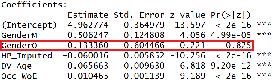
Multiple Logistic Regression output in R

Interpretation of Model Summary Output

We have set the alpha for variable significance at 0.0001. The p-value of the Gender variable is more than 0.0001 as such we may accept the Null Hypothesis, i.e. the Gender variable may be considered as insignificant and should be dropped.
The beta coefficient of the independent variables is in line with their correlation trend with the dependent variable.
- HP_Imputed variable has a negative correlation with the Target phenomenon, hence it’s beta coefficient is negative,
- Whereas the other variables have a positive correlation and accordingly their beta coefficients have come positive.

Re-run after dropping Gender Variable

The Gender variable was insignificant in the above model run. As such, we drop the Gender variable and re-run the logistic function.

Content goes here

mylogit = sm.glm(
    formula = "Target ~ HP_Imputed + DV_Age + Occ_WoE", 
    data = dev, family = sma.families.Binomial()
).fit()

mylogit.summary()

	coef	std err	z	P>\|z\|	[0.025	0.975]
Intercept	-4.1712	0.337	-12.387	0.000	-4.831	-3.511
HP_Imputed	-0.0625	0.006	-10.815	0.000	-0.074	-0.051
DV_Age	0.0567	0.009	6.132	0.000	0.039	0.075
Occ_WoE	0.0101	0.001	10.437	0.000	0.008	0.012

mylogit <- glm( 
  formula = Target ~ HP_Imputed + DV_Age + Occ_WoE, 
  data = dev, family = "binomial"
)
summary(mylogit)

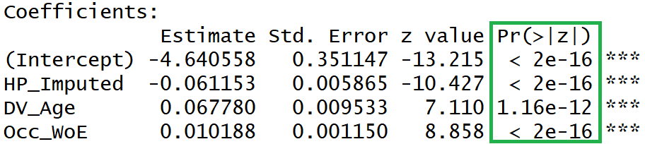
Multiple Logistic Regression Summary Output

All the variables are now significant.

Predict Probabilities

# predict code in python
dev["prob"] = mylogit.predict(dev)

# predict code in R

dev$prob <- predict(mylogit, dev, type="response")

Model Performance Measurement

How good is our model? Is the model usable? Is the model a good fit?
To answer these questions we have to measure the model performance.
(I suggested reading our blog on 7 Important Model Performance Measures before executing the below code)

Rank Order, KS, Gains Table & Lift Chart

dev['decile']=pd.qcut(dev.prob, 10, labels=False)

def Rank_Order(X,y,Target):
    
    Rank=X.groupby('decile').apply(lambda x: pd.Series([
        np.min(x[y]),
        np.max(x[y]),
        np.mean(x[y]),
        np.size(x[y]),
        np.sum(x[Target]),
        np.size(x[Target][x[Target]==0]),
        ],
        index=(["min_prob","max_prob","avg_prob",
                "cnt_cust","cnt_resp","cnt_non_resp"])
        )).reset_index()
    Rank=Rank.sort_values(by='decile',ascending=False)
    Rank["rrate"]=round(Rank["cnt_resp"]*100/Rank["cnt_cust"],2)
    Rank["cum_cust"]=np.cumsum(Rank["cnt_cust"])
    Rank["cum_resp"]=np.cumsum(Rank["cnt_resp"])
    Rank["cum_non_resp"]=np.cumsum(Rank["cnt_non_resp"])
    Rank["cum_cust_pct"]=round(Rank["cum_cust"]*100/np.sum(Rank["cnt_cust"]),2)
    Rank["cum_resp_pct"]=round(Rank["cum_resp"]*100/np.sum(Rank["cnt_resp"]),2)
    Rank["cum_non_resp_pct"]=round(
            Rank["cum_non_resp"]*100/np.sum(Rank["cnt_non_resp"]),2)
    Rank["KS"] = round(Rank["cum_resp_pct"] - Rank["cum_non_resp_pct"],2)
    Rank["Lift"] = round(Rank["cum_resp_pct"] / Rank["cum_cust_pct"],2)
    Rank
    return(Rank)


Gains_Table = Rank_Order(dev,"prob","Target")
Gains_Table

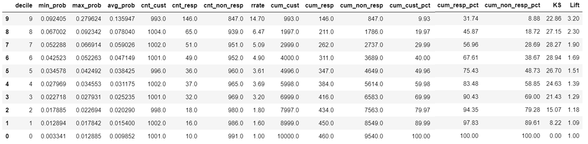
Rank Order, K-S Statistic, Gains Table and Lift Chart

Shown above is Gains Table output. The “rrate” (response rate) column shows that the model is Rank Ordering with a minor crack between decile number 5 & 4. The K-S statistic of the model is 0.2894 (28.94%). The Lift in the topmost decile is 3.20.

AUC-ROC

from sklearn.metrics import roc_curve

import matplotlib.pyplot as plt

%matplotlib inline

fpr, tpr, thresholds = roc_curve(dev["Target"],dev["prob"] )

plt.figure(figsize=(9,5))

plt.plot([0, 1], [0, 1], 'k--', label = 'Random')

plt.plot(fpr, tpr, color = 'blue', label = 'ROC')

plt.xlabel('False Positive Rate', fontsize=15)

plt.ylabel('True Positive Rate', fontsize=15)

plt.title('ROC Curve', fontsize=20)

plt.legend(fontsize=10, loc='best')

plt.show()

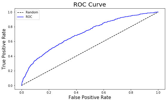
Multiple Logistic Regression AUC-ROC Model Performance Measure

from sklearn.metrics import  auc
roc_auc = round(auc(fpr, tpr), 3)

KS = round((tpr - fpr).max(), 3)


print("AUC of the model is:", roc_auc)
print("KS of the model is:", KS)

AUC of the model is: 0.707
KS of the model is: 0.297

The AUC of the model is 0.70. Based on AUC’s interpretation, the model may be considered to be a poor or just fair model.

Gini Coefficient

gini_coeff = 2 * roc_auc - 1

print("AUC of the model is:", roc_auc)

Gini Coefficient of the model is: 0.414

Hosmer-Lemeshow Goodness of Fit Test

#Hosmer-Lemeshow Goodness of Fit Function
def chisq(data,groupby,obs,Exp):

    chisq_tbl=data.groupby(groupby).apply(lambda x: pd.Series([

        np.size(x[obs]),

        np.size(x[Exp][x[Exp]==1]),

        np.size(x[Exp][x[Exp]==0]),

        np.sum(x[obs]),
        (np.sum(1-x[obs]))      
        ],
        index=(["cnt", "Obs_Resp", "Obs_Non_resp", 
               "Exp_Resp", "Exp_Non_Resp"])
        )).reset_index()
    chisq_tbl=chisq_tbl.sort_values(by=groupby,ascending=False)
    chisq_value = (
        ((chisq_tbl["Obs_Resp"]-chisq_tbl["Exp_Resp"])**2
              /chisq_tbl["Exp_Resp"])+
        ((chisq_tbl["Obs_Non_resp"]-chisq_tbl["Exp_Non_Resp"])**2
              /chisq_tbl["Exp_Non_Resp"])).sum()
    
    g = len(data["decile"].value_counts())
    
    
    chisq_tbl = chisq_tbl.round(0).astype(int)
    import scipy
    pvalue=scipy.stats.chi2.pdf(chisq_value , g-2)
    return({"Chisq_Table":chisq_tbl,
            "hosmerlem": {"degree_of_freedom": g-2,
                          "X^2":round(chisq_value,2),
                          "p_value":round(pvalue, 5)}})

chisq_test = chisq(dev, "decile", "prob", "Target")

chisq_test["Chisq_Table"]

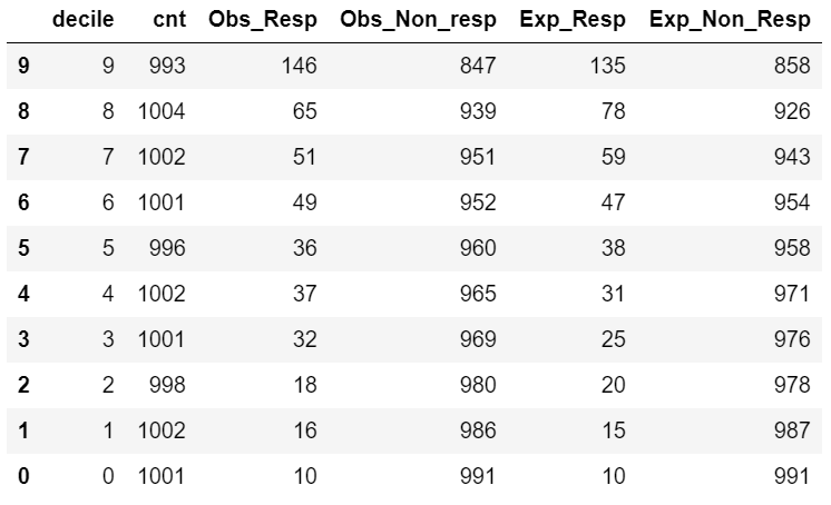
chisq_test["hosmerlem"]

{'degree_of_freedom': 8, 'X^2': 8.13, 'p_value': 0.09606}

The p-value of the HL-GOF test is above 0.05. We may accept the Null Hypothesis, i.e., the model fits the data very well.

Practice Exercise

The KS, AUC, Gini Coefficient of the above model suggests that the model is just fair. It is not a very good model. Improving the above model is an exercise for the blog reader.
Remember, in the above regression, we have not used the Balance, No. of Credit Transactions, and SCR variable. Try to bring these variables into the model and improve the overall model performance.
We used the Occ_WoE variable in the above model, however, we could have used the Occ_Imputed or Occ_KNN_Imputed imputed variables as created in the Missing Value Imputation step.

<<< previous blog | next blog >>>
Logistic Regression blog series home