How do you evaluate a machine learning model?
In Machine Learning, there are various metrics to evaluate the performance of a model and gauge its efficacy. In this blog series, we will learn 7 important model performance measures that can be used for the evaluation of a Binary Classification Model. They are:
- Rank Order table and Kolmogorov-Smirnov (K-S) Statistic
- Gains Table & Lift Chart
- Classification Accuracy
- AUC-ROC
- Concordance – Discordance
- Gini Coefficient
- Hosmer-Lemeshow Goodness of Fit
Examples of Binary Classification Business Problems
- Whether a customer will respond (not respond) to the marketing offer?
- Will a loan customer default (not default)?
- How likely is that a particular employee will resign (not resign)?
- What is the possibility of an insurance policyholder lapsing his premium payment?
- How likely is a retail chain customer will churn?
- How likely is a telecom subscriber will churn?
Of the 7 important model performance measures, I have used Rank Order and K-S statistics the most. The implementation strategy of many predictive models is designed based on the Rank Order table. As such, a Data Scientist must understand it.
Rank Order table
Rank Order Table is a key model performance measure used to evaluate how well the model separates the binary classes, viz, Responder class from Non-Responders, Defaulters from Non-Defaulters, Churners from Non-Churners, etc.
Let us quickly understand how to create the Rank Order table:
Step 1: Predict Probability
Apply the predictive model on the labeled data. Predict the probability for each record using the model. Your dataset would be something as shown in the below table:
| ID | PV1 | PV2 | PV3 | … | … | … | PVn | Target | Probability |
| 1 | … | .. | .. | …… | 0 | 0.0562 | |||
| 2 | .. | . | .. | …… | 0 | 0.1345 | |||
| . | …… | .. | .. | …… | 0 | … | |||
| . | …. | …. | .. | …… | 1 | 0.5122 | |||
| . | …… | … | .. | 0 | … | ||||
| .. | .. | .. | …… | 0 | … | ||||
| n | … | … | .. | …… | 1 | … |
Field description
ID: Unique Identifier
PV1 to PVn: Predictor Variables
Target: Labeled class column having values as 1 and 0. Let us say all 1s are Responder Class and all 0s are Non-responder Class
Probability: The probability of record belonging to Responder Class, i.e. Target = 1
Step 2: Rank (Decile) the data
Sort the data by Probability. Let us assume we have done ascending sort.
Split the data into 10 equal parts and rank them as 1 to 10. Rank 1 be assigned to the group with the lowest probability and Rank 10 to the group with the highest probability.
Decile
Step 3: Aggregate the data
Aggregate the data by Rank and get the count of customers, count responders, and count non-responders. On aggregation, the summarized data should be as shown in the table below.
| Decile (Rank) | # Customers |
# Responders |
# Non-Resp. |
| 10 | 1,000 | 295 | 705 |
| 9 | 1,000 | 176 | 824 |
| 8 | 1,000 | 115 | 885 |
| 7 | 1,000 | 75 | 925 |
| 6 | 1,000 | 35 | 965 |
| 5 | 1,000 | 30 | 970 |
| 4 | 1,000 | 23 | 977 |
| 3 | 1,000 | 18 | 982 |
| 2 | 1,000 | 13 | 987 |
| 1 | 1,000 | 7 | 993 |
| Total | 10,000 | 787 | 9,213 |
Step 4: Compute Response Rate
Response Rate is computed by taking the ratio of # Responders to # Customers.
| Decile (Rank) | # Customers |
# Responders |
# Non-Resp. |
% Resp. Rate |
| 10 | 1,000 | 295 | 705 | 29.5% |
| 9 | 1,000 | 176 | 824 | 17.6% |
| 8 | 1,000 | 115 | 885 | 11.5% |
| 7 | 1,000 | 75 | 925 | 7.5% |
| 6 | 1,000 | 35 | 965 | 3.5% |
| 5 | 1,000 | 30 | 970 | 3.0% |
| 4 | 1,000 | 23 | 977 | 2.3% |
| 3 | 1,000 | 18 | 982 | 1.8% |
| 2 | 1,000 | 13 | 987 | 1.3% |
| 1 | 1,000 | 7 | 993 | 0.7% |
| Total | 10,000 | 787 | 9,213 | 7.87% |
Step 5: Interpret Rank Order table
From the above rank order table, we observe:
- The Response Rate of 29.5% in Decile10 is the highest. Whereas, it is the least in Decile 1.
- The response rate is progressively descending from 29.5% to 0.7% and is ranking in-line with the decile numbers. Hence the name – RANK ORDER TABLE
The Rank Order table is used for designing the model implementation strategy, profitability analysis, and more. As such, it is essential to ensure that your model has a proper rank ordering. At times, minor cracks or breaks in the rank order may be acceptable. However, if there are any major whipsaws then, it is advisable to rebuild/recalibrate the model.
Why is the Rank Order table so important?
The Rank Order table is very important because the implementation strategy of most of the models is designed based on it. Assume the average campaign cost per customer is Rs. 10/- and the revenue per conversion is Rs. 150/-. The campaign will be profitable only if our campaign conversion is above 6.7% (=10/150). The decile wise profitability for the above Rank Order table is as shown below:
| Decile (Rank) | # Customers |
# Responders |
# Non-Resp. |
% Resp. Rate | Campaign Cost | Revenue | Profit |
| 10 | 1,000 | 295 | 705 | 29.5% | 1000 * 10 = 10000 |
295 * 150 = 44250 |
34250 |
| 9 | 1,000 | 176 | 824 | 17.6% | 10000 | 26400 | 16400 |
| 8 | 1,000 | 115 | 885 | 11.5% | 10000 | 17250 | 7250 |
| 7 | 1,000 | 75 | 925 | 7.5% | 10000 | 11250 | 1250 |
| 6 | 1,000 | 35 | 965 | 3.5% | 10000 | 5250 | -4750 |
| 5 | 1,000 | 30 | 970 | 3.0% | 10000 | 4500 | -5500 |
| 4 | 1,000 | 23 | 977 | 2.3% | 10000 | 3450 | -6550 |
| 3 | 1,000 | 18 | 982 | 1.8% | 10000 | 2700 | -7300 |
| 2 | 1,000 | 13 | 987 | 1.3% | 10000 | 1950 | -8050 |
| 1 | 1,000 | 7 | 993 | 0.7% | 10000 | 1050 | -8950 |
| Total | 10,000 | 787 | 9,213 | 7.87% | 100000 | 118050 | 18050 |
From the above table, it is clear that overall profitability is just Rs. 18050. However, if we target the deciles 10 to 7 then the profitability is Rs. 59150/- (= 34250 + 16400 + 7250 + 1250). By targeting just 40% of the overall base we get 3.3X (= 59150 / 18050) times higher profitability.
Kolmogorov Smirnov (K-S)
Kolmogorov-Smirnov (K-S) statistic measures how well the binary classifier model separates the Responder class (Yes) from Non-Responder class (No). The range of K-S statistic is between 0 and 1. Higher the value better the model in separating the Responder class from Non-Responder class.
K-S Statistic Calculation
Shown below is the K-S statistic calculations. The K-S column is computed as the difference of % Cum. Resp. and % Cum. Non-Resp. The point of maximum separation is the K-S statistic.
| Rank | # Cust. |
# Resp. |
# Non-Resp. |
% Resp. Rate | Cum. Resp. | Cum. Non-Resp. | % Cum. Resp. | % Cum. Non-Resp. | K-S |
| 10 | 1,000 | 295 | 705 | 29.5% | 295 | 705 | 37.5% | 7.7% | 29.8% |
| 9 | 1,000 | 176 | 824 | 17.6% | 471 | 1529 | 59.8% | 16.6% | 43.3% |
| 8 | 1,000 | 115 | 885 | 11.5% | 586 | 2414 | 74.5% | 26.2% | 48.3% |
| 7 | 1,000 | 75 | 925 | 7.5% | 661 | 3339 | 84.0% | 36.2% | 47.7% |
| 6 | 1,000 | 35 | 965 | 3.5% | 696 | 4304 | 88.4% | 46.7% | 41.7% |
| 5 | 1,000 | 30 | 970 | 3.0% | 726 | 5274 | 92.2% | 57.2% | 35.0% |
| 4 | 1,000 | 23 | 977 | 2.3% | 749 | 6251 | 95.2% | 67.8% | 27.3% |
| 3 | 1,000 | 18 | 982 | 1.8% | 767 | 7233 | 97.5% | 78.5% | 19.0% |
| 2 | 1,000 | 13 | 987 | 1.3% | 780 | 8220 | 99.1% | 89.2% | 9.9% |
| 1 | 1,000 | 7 | 993 | 0.7% | 787 | 9213 | 100% | 100% | 0% |
| Total | 10,000 | 787 | 9,213 | 7.87% | 787 | 9213 | 100% | 100% | 0% |
Interpretation of Kolmogorov-Smirnov statistic
- In the above table, the maximum separation between the Responder and Non-Responder class is 48.3%. So the K-S statistics is 0.483
- The range of K-S value is from 0 to 1. It is desirable to have a K-S statistic between 0.45 to 0.70 for a good model, especially marketing models.
- If the K-S value is below 0.45 then, the model may have weak to moderate separation power.
- If the K-S value exceeds 0.7 then, there is a risk of overfitting and one should be cautious. It is advisable to do a stringent quality check of calculations, assumptions, hypothesis, data, etc before accepting the model having K-S of 0.7 or more.
Gains Table & Lift Chart
Gains table and Lift chart are used to measure how much gain/lift we can expect by using a predictive model vis-a-vis not using the model. Lift is calculated by taking a ratio of model strategy success rate to a random strategy success rate.
Lift Calculation
From the above Rank Order table, we see
- Total number of customers = 10000
- Total number of Responders = 787
- Response Rate = 787 / 10000 = 7.87%
Random strategy: Assume you randomly select a sample of 1000 customers for a marketing campaign. How many responders would you expect?
Ans: Approx 78 or 79 responders.
Model-based strategy: You target 1000 customers from the topmost decile, i.e Decile 10. How many responders would you expect?
Ans: Approx 295 responders.
What will be the lift? The lift will be 3.75 (Lift = 295 / 78).
Lift Definition: Lift is defined as the ratio of the success rate you get by the model strategy to the random strategy.
Gains Table
The term Gains means how much we have gained?
E.g. How many Responders we would gain if we consider the top 3 deciles (decile 10, 9, and 8)?
From the table below, we would have gained 74.5% (= 586 / 787) of the total responders.
Gains definition: Gains at a given decile is the ratio of the cumulative number of responders up to that decile divided by the total number of responders. See Gains table below for better understanding.
| Decile | # Cust. | # Resp. |
Cum. Cust. | %Cum. Cust. | Cum. Resp. | % Resp. | Cum. Gains | Lift |
| 10 | 1,000 | 295 | 1000 | 10% | 295 | 37.5% | 37.5% | 3.75 |
| 9 | 1,000 | 176 | 2000 | 20% | 471 | 22.3% | 59.8% | 2.99 |
| 8 | 1,000 | 115 | 3000 | 30% | 586 | 14.6% | 74.5% | 2.48 |
| 7 | 1,000 | 75 | 4000 | 40% | 661 | 9.5% | 84.0% | 2.10 |
| 6 | 1,000 | 35 | 5000 | 50% | 696 | 4.5% | 88.4% | 1.77 |
| 5 | 1,000 | 30 | 6000 | 60% | 726 | 3.8% | 92.2% | 1.54 |
| 4 | 1,000 | 23 | 7000 | 70% | 749 | 2.9% | 95.2% | 1.36 |
| 3 | 1,000 | 18 | 8000 | 80% | 767 | 2.2% | 97.5% | 1.22 |
| 2 | 1,000 | 13 | 9000 | 90% | 780 | 1.7% | 99.1% | 1.10 |
| 1 | 1,000 | 7 | 10000 | 100% | 787 | 0.9% | 100% | 1 |
| Total | 10,000 | 787 |
From the above table, if we target only the customers in the top decile (i.e decile 10) then, we would target 10% of the total customers. In that decile, we get 37.5% of the total responders. The ratio of 37.5% / 10% is the LIFT.
Let us take one more example to understand it better. If we target the top 3 deciles (i.e decile 10, 9, and 8) then, we would be targetting 30% of the total customers. However, we gain 74.5% of the total responders in the top 3 deciles. The ratio of 74.5% / 30% = 2.48 is the Lift.
In short, Lift is defined as Cumulative Gains divided by % Cumulative Customers. As a benchmark, a good marketing model should have a lift of 3.5 and more in the topmost decile.
Lift Chart & its Interpretation
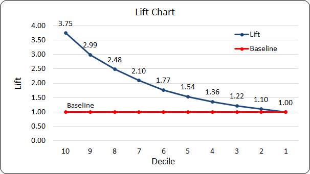
- If we target only the customers in topmost decile, i.e Decile No 10, we will get a lift of 3.75
- The lift of the cumulative of the top 2 deciles is 2.99.
- If all the deciles are considered then, the lift will be 1. A lift of 1 means there is no gain vis-a-vis the baseline.
Python Code for K-S, Gains Table & Lift Chart
Assume you have a dataset named “dev” with dependent variable “Target” having values 1 & 0 to indicate Responder & Non-Responder respectively. The model estimated probability is in the column “prob”. The Python code for Rand Order, K-S, Gains table & Lift calculation is given below.
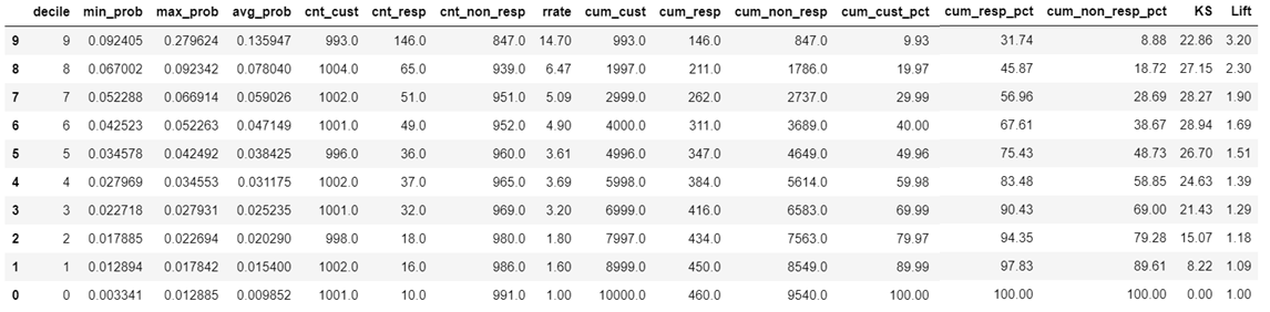
dev['decile']=pd.qcut(dev.prob, 10, labels=False)

def Rank_Order(X,y,Target):

    Rank=X.groupby('decile').apply(lambda x: pd.Series([
        np.min(x[y]),
        np.max(x[y]),
        np.mean(x[y]),
        np.size(x[y]),
        np.sum(x[Target]),
        np.size(x[Target][x[Target]==0]),
        ],
        index=(["min_prob","max_prob","avg_prob",
                "cnt_cust","cnt_resp","cnt_non_resp"])
        )).reset_index()
    Rank=Rank.sort_values(by='decile',ascending=False)
    Rank["rrate"]=round(Rank["cnt_resp"]*100/Rank["cnt_cust"],2)
    Rank["cum_cust"]=np.cumsum(Rank["cnt_cust"])
    Rank["cum_resp"]=np.cumsum(Rank["cnt_resp"])
    Rank["cum_non_resp"]=np.cumsum(Rank["cnt_non_resp"])
    Rank["cum_cust_pct"]=round(Rank["cum_cust"]*100/np.sum(Rank["cnt_cust"]),2)
    Rank["cum_resp_pct"]=round(Rank["cum_resp"]*100/np.sum(Rank["cnt_resp"]),2)
    Rank["cum_non_resp_pct"]=round(
            Rank["cum_non_resp"]*100/np.sum(Rank["cnt_non_resp"]),2)
    Rank["KS"] = round(Rank["cum_resp_pct"] - Rank["cum_non_resp_pct"],2)
    Rank["Lift"] = round(Rank["cum_resp_pct"] / Rank["cum_cust_pct"],2)
    Rank
    return(Rank)


Gains_Table = Rank_Order(dev,"prob","Target")
Gains_Table
Shown below is sample Gains Table output. (Reference Read: Logistic Regression Model Performance Measures). The “rrate” (response rate) column shows that the model is Rank Ordering with a small crack between decile 5 & 4. The K-S statistic of the model is 0.2894 (28.94%) and Lift in the topmost decile is 3.20.
Next Blog
In the upcoming blog, we will discuss the Classification Accuracy & AUC-ROC Curve model performance measures.
Is this specific to marketing campaign strategies? Which other domains can these be implemented?
Perhaps in specific domains – the nonresponders would be the focus – lets say in a hospital environment – where particular category of patients not responding to treatment. How would we measure the KS / RO tables?
The calculation of KS / RO remains the same. According to the phenomenon of interest to you, you will have to define the Target Variable. For e.g if non-responders is the phenomenon of your interest then, define Target = 1 for non-responders and Target = 0 for responders. I hope this helps. Thanks.
Excellent Article.Lucid Explanation of the concepts.Only thing i would like to see is cumulative gain code in final python code.
Is it a must that the ks gets captured in the first 3 deciles?
What if it’s in the 5th decile , 8th decile ?
Ideally yes. However, we may get the KS in 4th or 5th decile if the predictor variables are weak.