Information Value and Weight of Evidence (WoE)

Information Value and Weight of Evidence (WoE) are the two most used concepts in Logistic Regression for variable selection and variable transformation respectively. Information Value helps quantify the predictive power of a variable in separating the Good Customers from the Bad Customers. Whereas, WoE is used for the transformation of categorical variables to continuous.

Pre-reads: Information Value and Variable Transformation

Understanding WoE Calculations

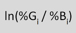
WoE is calculated by taking the natural logarithm (log to base e) of the ratio of %Good by %Bad.

Weight of Evidence Formula

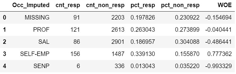
The table below shows the Weight of Evidence calculations for the Occupation field. I will walk you through step-by-step calculations to compute WoE.

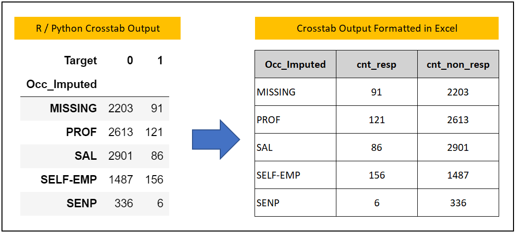
Step 1: Get the frequency count of the dependent variable class by the independent variable. This step will give the first three columns of the above table.

• Occ_Imputed: Independent Varible.
• cnt_resp: Count of Responders, i.e Target = 1
• cnt_non_resp: Count of Non-Responders i.e Target = 0

# Crosstab code in Python

pd.crosstab(dev["Occ_Imputed"], dev["Target"])

# Crosstab code in R 
table(dev$Occ_Imputed, dev$Target)

# Note - The Development Sample of R and Python is not exactly the same. 
# As such, you can expect some difference in R and Python crosstab output.

Step 2: Convert the count values into proportions. The formula is count responders divided by total responders and likewise count non-responders divided by total non-responders.

Step 3: Calculate WoE by taking the natural log of the ratio of Responders proportion divided by Non-Responders.

Python code to compute WoE

We have automated the above WoE calculation in the k2_iv_woe_function.py file. You can download the k2_iv_woe_function.py file from Github.

exec(open("k2_iv_woe_function.py").read())
woe_table = woe(df=dev, target="Target",var="Occ_Imputed",
   bins = 10, fill_na = True)
woe_table

Application of WoE for Variable Transformation

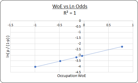
The WoE can be used to transform Categorical Variable to Numerical. You do this by substituting each category by their respective WoE value. The benefit of WoE transformation is that the WoE transformed variable has a linear relationship with the log odds. To understand it better, execute the below code and see its Ln Odds Visualization chart.

# All WOE values has been multiplied by 100


dev["Occ_WoE"]=dev["Occ_Imputed"].map(lambda
         x: -15.469 if (x == "MISSING")
         else (-4.044 if (x == "PROF")
         else (-48.644 if (x == "SAL")
        else (77.736 if (x == "SELF-EMP")
        else -99.333     
              ))))

# All WOE values has been multiplied by 100
dev$Occ_WoE = ifelse(

  dev$Occ_Imputed == "MISSING", 8.94,

    ifelse (dev$Occ_Imputed == "PROF", -10.92,

      ifelse (dev$Occ_Imputed  == "SAL", -50.77,

        ifelse (dev$Occ_Imputed == "SELF-EMP",65.82,  -81.37

          ))))

Benefits of using WoE in Logistic Regression

1. Does away with One-Hot Encoding: Some of the machine learning packages do not take the categorical variables directly. You have to convert the categorical variables into a dummy 1-0 matrix also called one-hot encoding. If there are many categories in the categorical variable then, it would add many columns in the dataset. We can do away with the one-hot encoding by using the WoE step.

2. Only One Beta Coefficient: A categorical variable with “n” categories will result in having “n-1” beta coefficients in the model. However, converting a categorical variable to its WoE equivalent will have only one beta coefficient thereby simplifying the model equation.

<<< previous blog         |         next blog >>>
Logistic Regression blog series home