A single categorical variable is mostly analyzed by Frequency Distribution.
A table or a graph displaying the occurrence frequency of various outcomes is called Frequency Distribution. The commonly used tabular and graphical methods for frequency distribution analysis are:
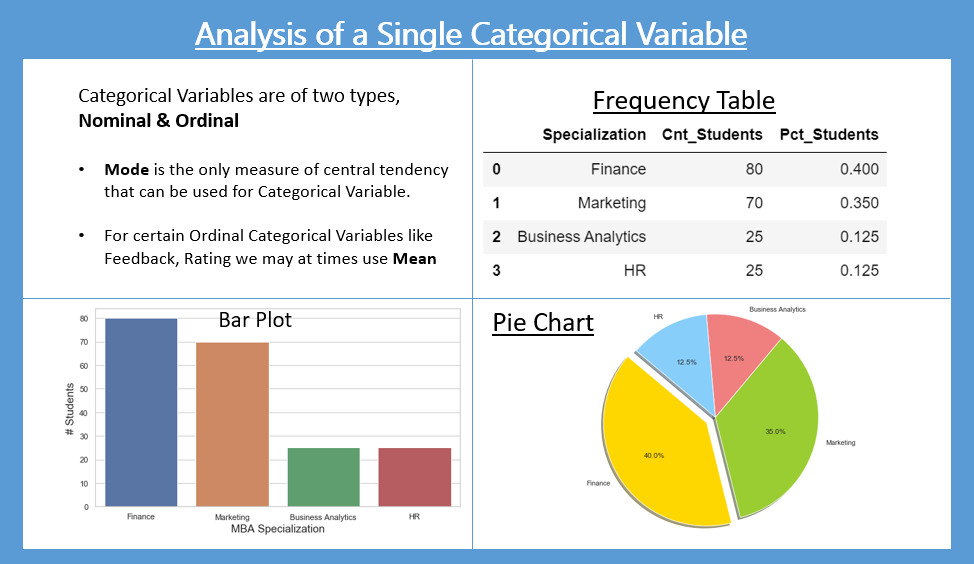
- Frequency Table is used to show the frequency distribution in tabular form.
- Bar Plot is used to show the frequency distribution in a visual format.
- Pie Chart to show the distribution in proportions. Proportions help us compare parts of a whole.
Let’s take the example of “MBA Students” data to learn more about frequency distribution analysis. (read the previous blog link)
Data Import
# Import the required packages
import pandas as pd
import os
import matplotlib.pyplot as plt
import seaborn as sns
%matplotlib inline
# set directory as per your file folder path
os.chdir("d:/k2analytics/datafile")


# read the file
mba_df = pd.read_csv("MBA_Students_Data.csv")
#Set directory as per your folder file path
setwd("D:/k2analytics/datafile")
getwd()

#Read the File

mba_df = read.csv("MBA_Students_Data.csv", header = TRUE)
Frequency Distribution Analysis of the MBA Specialization field
We would like to know the frequency distribution of the MBA Students by their choice of Specialization. This information is captured in the variable – “mba_specialization” and it is of type – “categorical”. To be more specific, mba_specialization is of Nominal Variable type.
We can summarize the “mba_specialization” by using Frequency Distribution Table, Proportions, Bar Plot, Pie Chart.
Tabular Methods: Frequency Distribution Table
freq_table = mba_df["mba_specialization"].value_counts().to_frame()
freq_table.reset_index(inplace=True) # reset index
freq_table.columns = [   "Specialization"   , "Cnt_Students"] # rename columns
freq_table["Pct_Students"] = freq_table["Cnt_Students"] / sum(freq_table["Cnt_Students"])
freq_table
| Specialization |
Cnt_Students |
Pct_Students |
| Finance |
80 |
0.400 |
| Marketing |
70 |
0.350 |
| Business Analytics |
25 |
0.125 |
| HR |
25 |
0.125 |
| Total |
200 |
1 |
R code for Frequency Distribution
freq_table = transform(table(mba_df$mba_specialization))
freq_table = freq_table[order(freq_table$Freq, decreasing = TRUE),]

names(freq_table) = c("Specialization","Cnt_Students")

rownames(freq_table) = 1:nrow(freq_table)

freq_table$Per_Students = freq_table$Cnt_Students/sum(freq_table$Cnt_Students)

freq_table
| Specialization |
Cnt_Students |
Pct_Students |
| Finance |
80 |
0.400 |
| Marketing |
70 |
0.350 |
| Business Analytics |
25 |
0.125 |
| HR |
25 |
0.125 |
Numerical Methods: Mode
The Mode is the only measure of central tendency which can be used for Nominal Variables. From the above table, the Mode is 80 and the corresponding category for mode is Finance.
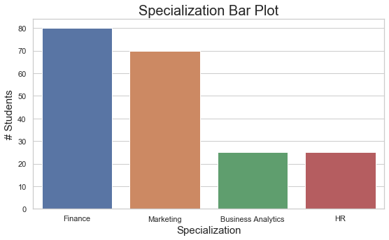
Graphical Methods: Bar plot
# Simple one line syntax to make bar plot
plt.bar(freq_table['Specialization'], freq_table['Cnt_Students'])
# Bar plot code with formatting and pretty look and feel
sns.set(style="whitegrid")
plt.figure(figsize=(9,5))
ax = sns.barplot( x = freq_table["Specialization"],
            y = freq_table["Cnt_Students"])
ax.axes.set_title("Specialization Bar Plot",fontsize=20)
ax.set_xlabel("Specialization",fontsize=15)
ax.set_ylabel("# Students",fontsize=15)
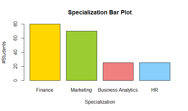
barplot(height = freq_table$Cnt_Students,
        names.arg = freq_table$Specialization,
        main = "Specialization Bar Plot",
        xlab = "Specialization",
        ylab = "#Students",
        col = c('gold', 'yellowgreen', 'lightcoral', 'lightskyblue')
        )
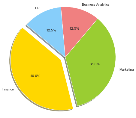
Graphical Methods: Pie Chart
# Python Pie Chart code with formatting
plt.figure(figsize=(7,7))
colors = ['gold', 'yellowgreen', 'lightcoral', 'lightskyblue']
explode = (0.1, 0, 0, 0)  # explode 1st slice

# Plot
plt.pie(freq_table['Cnt_Students'],
        labels=freq_table['Specialization'],
        explode=explode,
        colors=colors,
        autopct='%1.1f%%',
        shadow=True, startangle=140)

plt.axis('equal')
plt.show()
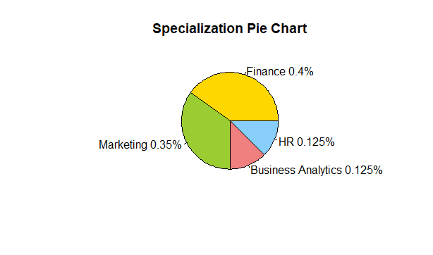
#Pie Chart

pie(
   x = freq_table$Cnt_Students,
   labels = paste(freq_table$Specialization," ",
   freq_table$Per_Students,"%",sep=""),
   col = c('gold', 'yellowgreen', 'lightcoral', 'lightskyblue'),
   main = 'Specialization Pie Chart'
)
Interpretation / Take away:
- 40% of the students are specializing in Finance.
- 35% of the students have chosen Marketing as their field of specialization
- HR and Business Analytics have 25 students each.
Graduation Degree
Let’s say, we wish to know the Graduation background of the students pursuing the MBA course. This information is captured in the variable – “grad_degree” and it is of type – “categorical”.
Tabular Methods: Frequency Distribution Table
The analysis of grad_degree as shown below shows that there are 45 distinct values. As the number of graduation degree categories are many, we should recategorize them. Recategorization is process of categorizing again, i.e., the act of assigning something to another category. E.g. B.E – Mechanical, B.E – Computers categories in our data can be recategorized as B.E.
freq_grad_deg = mba_dst['grad_degree'].value_counts()
freq_grad_deg.count()

Out[7] : 45
freq_grad_deg

Out[8] :
B.Com                                           65
B.M.S                                           31
B.E                                             18
B.A.F                                            9
B.E - Mechanical                                 9
B.Com - Honours                                  6
B.B.A                                            4
B.Tech                                           4
B.E - Computers                                  3
B.E - Civil                                      3
B.Sc                                             3
B.E - EXTC                                       3
B.Tech - Mechanical                              2
B.E - Electronics and Telecommunications         2
B.Com - Financial Markets                        2
B.E - Computer Engineering                       2
B.Tech - Computer Science                        2
B.E - Production Engineering                     2
Bachelor of Banking and Insurance                2
B.Sc - Information Technology                    2
B.E - Electrical                                 2
B.E - Information Technology                     1
B.E - Chemical                                   1
B.Sc - Nautical Science                          1
B.Sc - Aeronautics                               1
B.E, Mumbai University                           1
Bachelor In Engineering                          1
B.B.A - IT                                       1
B.Tech - Civil Infrastructure Engineering        1
B.E - Electronics                                1
B.Sc - Zoology                                   1
Bachelor of Banking and Finance                  1
B.Sc - Hotel Management                          1
B.E Production                                   1
B.M.M - Journalism                               1
B.Sc - Physics, Chemistry, Maths                 1
B.Sc - Hospitality and Hotel Administration      1
Bachelor in Computer Application                 1
B.Tech - EXTC                                    1
B.Sc - Computer Science                          1
B.E - ENTC                                       1
B.B.A - IB                                       1
B.E - CSE                                        1
B.B.I                                            1
B.M.M                                            1
Name: grad_degree, dtype: int64
Python function for recategorizing the graduation degree values.
def fn_grad_deg_recat(x):
    x = x.upper()
    if ("B.COM" in x
        or "B.A.F" in x
       ):
        return "B.Com / B.A.F"
    elif ("B.E" in x
          or "B.TECH" in x
          or x == "BACHELOR IN ENGINEERING"
          or x == "BACHELOR IN COMPUTER APPLICATION"
         ):
        return "B.E / B.Tech"
    elif "B.M.S" in x:
        return "B.M.S"
    elif "B.SC" in x:
        return "B.Sc"
    elif ("B.BA" in x
           or "B.B.A" in x
         ):
        return "B.B.A"
    else:
        return "Other Specializations"
mba_df['grad_deg_recat'] = mba_df['grad_degree'].map(fn_grad_deg_recat)
freq_grad_deg = mba_df['grad_deg_recat'].value_counts().to_frame()
freq_grad_deg.reset_index(inplace=True) # reset index
freq_grad_deg.columns = ["Graduation Degree" , "Cnt_Students"] # rename columns
freq_grad_deg["Pct_Students"] = freq_grad_deg["Cnt_Students"] / sum(freq_grad_deg['Cnt_Students'])
freq_grad_deg
|
Graduation Degree |
Cnt_Students |
Pct_Students |
| 0 |
B.Com / B.A.F |
82 |
0.410 |
| 1 |
B.E / B.Tech |
63 |
0.315 |
| 2 |
B.M.S |
31 |
0.155 |
| 3 |
B.Sc |
12 |
0.060 |
| 4 |
B.B.A |
6 |
0.030 |
| 5 |
Other Specializations |
6 |
0.030 |
freq_grad_deg = transform(table(mba_df$grad_degree))
nrow(freq_grad_deg)

#Output

> nrow(freq_grad_deg)
[1] 45
> print(freq_grad_deg)

                                           Var1 Freq
1                                         B.A.F    9
2                                         B.B.A    4
3                                    B.B.A - IB    1
4                                    B.B.A - IT    1
5                                         B.B.I    1
6                                         B.Com   65
7                     B.Com - Financial Markets    2
8                               B.Com - Honours    6
9                                           B.E   18
10                               B.E - Chemical    1
11                                  B.E - Civil    3
12                   B.E - Computer Engineering    2
13                              B.E - Computers    3
14                                    B.E - CSE    1
15                             B.E - Electrical    2
16                            B.E - Electronics    1
17     B.E - Electronics and Telecommunications    2
18                                   B.E - ENTC    1
19                                   B.E - EXTC    3
20                 B.E - Information Technology    1
21                             B.E - Mechanical    9
22                 B.E - Production Engineering    2
23                               B.E Production    1
24                       B.E, Mumbai University    1
25                                        B.M.M    1
26                           B.M.M - Journalism    1
27                                        B.M.S   31
28                                         B.Sc    3
29                           B.Sc - Aeronautics    1
30                      B.Sc - Computer Science    1
31 B.Sc - Hospitality and Hotel Administration     1
32                      B.Sc - Hotel Management    1
33                B.Sc - Information Technology    2
34                      B.Sc - Nautical Science    1
35             B.Sc - Physics, Chemistry, Maths    1
36                               B.Sc - Zoology    1
37                                       B.Tech    4
38    B.Tech - Civil Infrastructure Engineering    1
39                    B.Tech - Computer Science    2
40                                B.Tech - EXTC    1
41                          B.Tech - Mechanical    2
42             Bachelor in Computer Application    1
43                      Bachelor In Engineering    1
44              Bachelor of Banking and Finance    1
45            Bachelor of Banking and Insurance    2
R function for recategorizing the graduation degree values.
fn_grad_deg_recat = function(x){
        x = toupper(x)
        if (grepl("B.COM",x) || grepl("B.A.F",x)){
                return ("B.Com / B.A.F")
        }
        else if(grepl("B.M.S",x)){
                return ("B.M.S")
        }
        else if(grepl("B.E",x)
                || grepl("B.TECH",x)
                ||x == "BACHELOR IN ENGINEERING"
                ||x == "BACHELOR IN COMPUTER APPLICATION"){
                return ("B.E / B.Tech")
        }
        else if(grepl("B.SC",x)){
                return ("B.Sc")
        }
        else if (grepl("B.BA",x) || grepl("B.B.A",x) ){
                return ("B.B.A")
        }
        else{
                return("Other Specializations")
        }
}
mba_df$grad_deg_recat = lapply(mba_df$grad_degree, fn_grad_deg_recat)

# Converting List to Vector
mba_df$grad_deg_recat = as.vector(unlist(mba_df$grad_deg_recat))
freq_grad_deg_recat = transform(table(mba_df$grad_deg_recat))
freq_grad_deg_recat = freq_grad_deg_recat[order(freq_grad_deg_recat$Freq, decreasing = TRUE),]

# Renaming column names
names(freq_grad_deg_recat) = c("Graduation Degree","Cnt_Students")

# Reseting row index
rownames(freq_grad_deg_recat) = 1:nrow(freq_grad_deg_recat)

freq_grad_deg_recat$Pct_Students = freq_grad_deg_recat$Cnt_Students/sum(freq_grad_deg_recat$Cnt_Students)
freq_grad_deg_recat
|
Graduation Degree |
Cnt_Students |
Pct_Students |
| 1 |
B.Com / B.A.F |
82 |
0.410 |
| 2 |
B.E / B.Tech |
63 |
0.315 |
| 3 |
B.M.S |
31 |
0.155 |
| 4 |
B.Sc |
12 |
0.060 |
| 5 |
B.B.A |
6 |
0.030 |
| 6 |
Other Specializations |
6 |
0.030 |
Note: We could have also recategorized the graduation degree as Science, Commerce, and Arts.
Interpretation / Take away:
- 41% of the students are from B.Com or Accounting & Finance background
- 31.5% of the students have B.E. / B.Tech background. Another 6% are from B.Sc.
- B.M.S. is the third major category with 15.5% of students.
Practise Exercise
- Create the Bar Plot and Pie Chart for Graduation using the “grad_deg_recat” column.
- Draw inferences for the “gender” variable
- Recategorize “ten_plus_2_stream” variable and analyze.
Next Blog
In the next blog, we will learn to analyze a single continuous variable using Histogram and Density Plots.
<<< previous | next blog >>>
<<< statistics blog series home >>>
Recent Comments