Variable Transformation in Machine Learning

In machine learning, we apply Variable Transformation to improve the fit of the regression model on the data. The functions such as Natural Log, Exponential, Square, Square-Root, Inverse, Binning/Bucketing, or some business logic is commonly used to perform variable transformation. In this blog, we will see how a simple variable transformation step can improve the model performance by about 10%.

Multiple Linear Regression Model

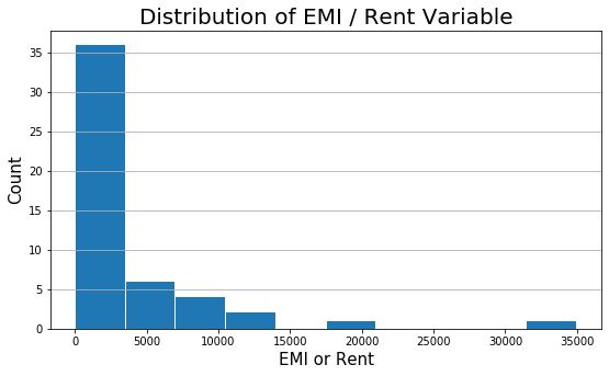
In the previous blog, we had built a multiple linear regression model using three variables, Mthly_HH_Income, No_of_Fly_Members, and Emi_or_Rent_Amt. The Adjusted R-Squared of the model is 0.678. Moreover, it was observed that there is skewness in the Emi_or_Rent_Amt variable. Shown below is the histogram plot of the Emi_or_Rent_Amt variable for quick remembrance.

plt.figure(figsize=(9,5))
plt.hist(inc_exp['Emi_or_Rent_Amt'], rwidth = 0.98)

plt.title("Distribution of EMI / Rent Variable", fontsize=20)
plt.xlabel('EMI or Rent', fontsize=15)
plt.ylabel('Count', fontsize=15)
plt.grid(axis='y')

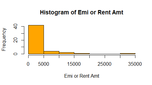
Variable Transformation of EMI Variable in Multiple Linear Regression Model

hist(x=inc_exp$Emi_or_Rent_Amt,  
     main = "Histogram of Emi or Rent Amt",
     xlab = "Emi or Rent Amt", 
     ylab = "Frequency",
     col = "orange")

Variable Transformation

From histogram, we see there is skeness in the variable Emi_or_Rent_Amt. I propose we should do a Natural Log transformation of the variable. The log normal functions will scale the variable and make it somewhat normally distributed.

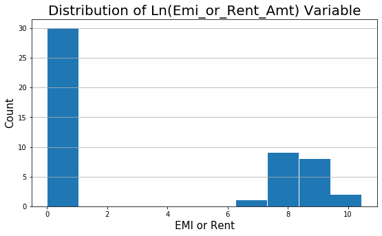
# Log Transformation step
import numpy as np
inc_exp['Ln_Emi_or_Rent_Amt'] = np.log(inc_exp['Emi_or_Rent_Amt'] + 1)

# Histogram
plt.figure(figsize=(9,5))
plt.hist(inc_exp['Ln_Emi_or_Rent_Amt'], rwidth = 0.98)

plt.title("Distribution of Ln(Emi_or_Rent_Amt) Variable", fontsize=20)
plt.xlabel('Ln (Emi_or_Rent_Amt)', fontsize=15)
plt.ylabel('Count', fontsize=15)
plt.grid(axis='y')

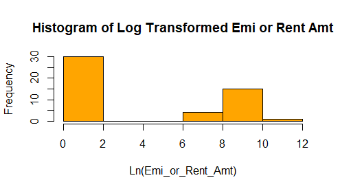
Variable Transformation Example in Linear Regression Machine Learning Model

inc_exp$Ln_Emi_or_Rent_Amt = log(inc_exp$Emi_or_Rent_Amt + 1)

hist(x=inc_exp$Ln_Emi_or_Rent_Amt ,  
     main = "Histogram of Log Transformed Emi or Rent Amt",
     xlab = "Ln(Emi_or_Rent_Amt)", 
     ylab = "Frequency",
     col = "orange")

Natural Log Transformation of EMI_Rent Variable in R

Model Performance Comparison

We will compare the model built with & without variable transformation to see the improvement in Adjusted R-Squared model performance measure.

## Multiple Linear Regression Without Transformation
m_linear_mod = sma.ols(formula = "Mthly_HH_Expense ~ Mthly_HH_Income+\
                      No_of_Fly_Members + Emi_or_Rent_Amt  ",
                      data = inc_exp).fit()

## Multiple Linear Regression With Transformation
m_linear_mod_2 = sma.ols(formula = "Mthly_HH_Expense ~ Mthly_HH_Income+\
                      No_of_Fly_Members + Ln_Emi_or_Rent_Amt  ",
                      data = inc_exp).fit()

print("Adj. R-Squared WITHOUT Transformation", 
       m_linear_mod.rsquared_adj.round(4))

print("Adj. R-Squared WITH Transformation", 
       m_linear_mod_2.rsquared_adj.round(4))

Adj. R-Squared WITHOUT Transformation 0.6781
Adj. R-Squared WITH Transformation 0.7436

## Multiple Linear Regression Without Transformation

m_linear_mod <- lm( Mthly_HH_Expense ~ Mthly_HH_Income 
                    + No_of_Fly_Members + Emi_or_Rent_Amt, 
                    data = inc_exp )

## Multiple Linear Regression With Transformation

m_linear_mod_2 <- lm( Mthly_HH_Expense ~ Mthly_HH_Income 
                    + No_of_Fly_Members + Emi_or_Rent_Amt, 
                    data = inc_exp )

cat("Adj. R-Squared WITHOUT Transformation",
     summary(m_linear_mod)$adj.r.squared)


cat("Adj. R-Squared WITH Transformation",
    summary(m_linear_mod_2)$adj.r.squared)

Adj. R-Squared WITHOUT Transformation 0.6780635
Adj. R-Squared WITH Transformation 0.7435739

Note:

In linear regression, there is no assumption that the explanatory (independent) variable should be normally distributed. However, the model performance is improved significantly by transforming a skewed independent variable and making it normally distributed.

Practice Exercise

We have used only the initial 3 explanatory variables. The variables Highest_Qualified_Member & No_of_Earning_Member has been left as a practice exercise.

Next Blog

In the next blog, we will learn how to predict the estimated value, compute residuals (error), RMSE, and more.

<<< previous blog | next blog >>>
Linear Regression blog series home

Variable Transformation in Machine Learning

Multiple Linear Regression Model

Variable Transformation

Model Performance Comparison

Note:

Practice Exercise

Next Blog

Submit a Comment Cancel reply

Recent Posts

Recent Comments

Share This