
“R Squared” is a statistical measure that represents the proportion of variance in the dependent variable as explained by the independent variable(s) in regression. R Squared statistic evaluates how good the linear regression model is fitting on the data. In this blog, you will get a detailed explanation of the formula, concept, calculation, and interpretation of R Squared statistic.
Pre-read: Simple Linear Regression
R Squared Concept and Formula
R-Squared is also known as the Coefficient of Determination. The value of R-Squared ranges from 0 to 1. The higher the R-Squared value of a model, the better is the model fitting on the data. However, if the R-Squared value is very close to 1, then there is a possibility of model overfitting, which should be avoided. A good model should have an R-Squared above 0.8.
Related Reading: Adjusted R-Squared
Understanding the R Squared Concept
Assume, you have been provided with data of 500 Households. The data contains Monthly Income & Expense details of the households. The mean (arithmetic average) monthly expense of the households is Rs. 18818/-.
Assume there is Household X. You have been asked – What is the monthly expense of Household X?
- Scenario 1: You do not have any information about the household. In the absence of any data, your best guess estimate would be Rs. 18818/- i.e, the mean estimate.
- Scenario 2: The monthly income of the household is Rs. 10000/-. What will be your estimate now? It will obviously be a number far below the mean.
- Scenario 3: The monthly income of the household is Rs. 50000/-. Your estimate of the monthly expense will definitely be above the mean.
In short, if we do not have any information, then we rely on the mean estimate. If some information is available, then we can make a more accurate estimate as against relying on the mean estimate. “More Accurate” means “Less Error”. The mathematical quantification of this accuracy (or reduction in error) is R-Squared.
R Squared Formula
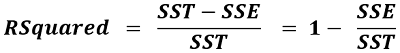
R Squared is a statistical measure that represents the proportion of variance in the dependent variable as explained by the independent variable(s).
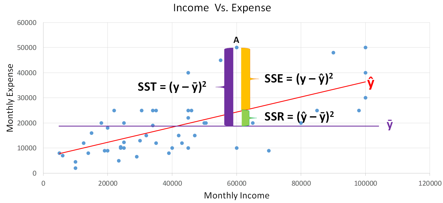
We will understand each of the above terms and their formulae using the Monthly Household Income vs. Expense scatter plot shown below:
Terminologies, Notations, and Formulae:
| Terminology | Notation / Formula | Description |
| Actual Value of Dependent Variable | y | The symbol y denotes the actual value of the dependent variable (in above plot y represents the Monthly Expense variable) |
| Independent Variable Value | x | The variable which is used to estimate the value of the dependent variable is called an independent variable (in above plot x represents the Monthly Income variable) |
| Mean of Dependent Variable | ȳ | The mean statistic of the dependent variable. The (purple line) in the above plot represents the mean of the Monthly Expense |
| Predicted (Estimated) Value | ŷ (y-cap) | The symbol ŷ denotes the model predicted value of the dependent variable. The predicted values are on the Line of Best Fit shown in red colour in the above plot |
| SST | 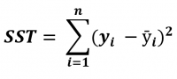 |
Sum of Squared Total (SST) is the square of the difference between the observed dependent variable and its mean. |
| Error | e = y – ŷ | Error is the difference between the actual and predicted (estimated) value. Error is also called Residual |
| Squared Error | (y – ŷ)^2 | Squared Error is simply the square of the error term, i.e. |
| SSE | 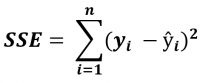 |
SSE is the Sum of Squared Errors. It is also called the Residual Sum of Squares (RSS) |
| SSR | 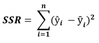 |
SSR is the Sum of Squared Regression. It is the error reduced because of the regression model. |
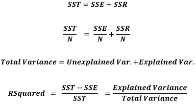
From the scatter plot, you can observe that SST = SSE + SSR. Note: SST / N is the same as the Variance formula, where N is the number of observations. Therefore by diving the LHS (Left Hand Side) and RHS (Right Hand Side) of the equation by N, we can express R Squared in terms of Variance.
Interpretation of R Squared in Linear Regression
# Import data
import pandas as pd
inc_exp = pd.read_csv("Inc_Exp_Data.csv")

#Build Model

import statsmodels.api as sm
xdat = inc_exp['Mthly_HH_Income']
xdat = sm.add_constant(xdat)
ydat = inc_exp['Mthly_HH_Expense']
model = sm.OLS(ydat, xdat).fit()
model.summary()

inc_exp <- read.csv("Inc_Exp_Data.csv")

linear_mod <- lm(
     formula = Mthly_HH_Expense ~ Mthly_HH_Income,
     data = inc_exp
)

summary(linear_mod)
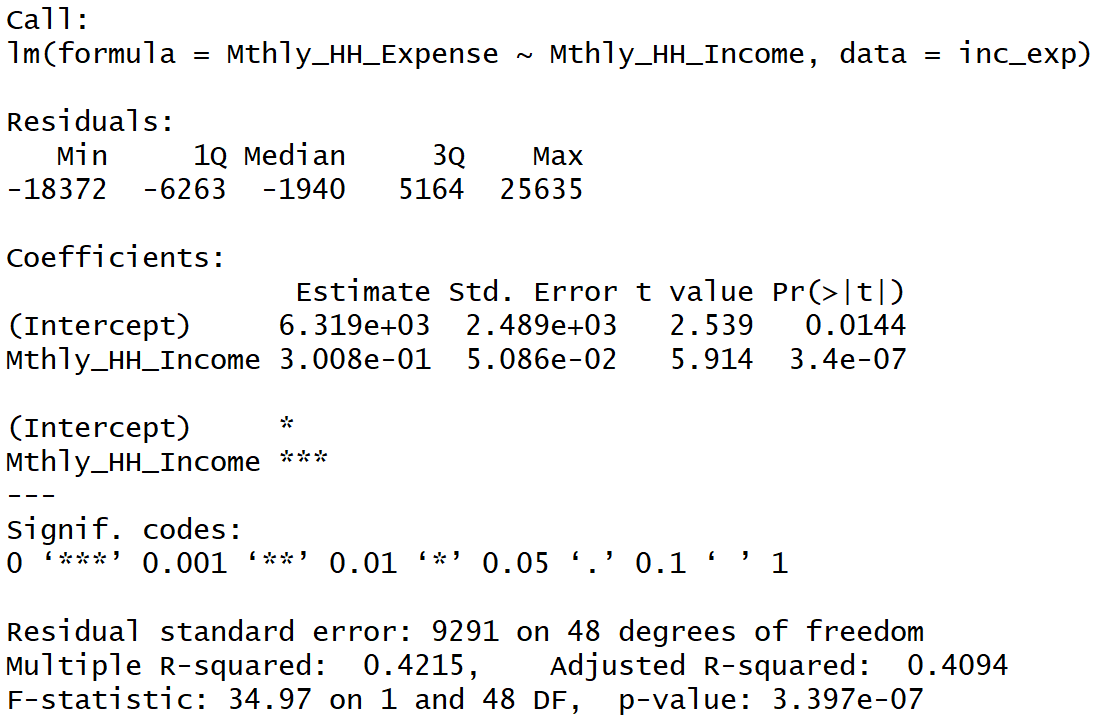
The R-Squared value of the simple linear regression model is 0.421. It signifies that 42.1% of the variance in the dependent variable (Mthly_HH_Expense) is explained by the independent variable (Mthly_HH_Income).
R Squared Calculation
Next Blog
In the next part of the Linear Regression blog series, we will learn about Multiple Linear Regression, Adjusted R-Squared, Multi-Collinearity, and more.
<<< previous blog | next blog >>>
Linear Regression blog series home
PS: Our Next Data Science Certification Program
Recent Comments