Multiple Linear Regression & Adjusted R-Squared

Multiple Linear Regression is a linear regression model having more than one explanatory variable. In our last blog, we discussed the Simple Linear Regression and R-Squared concept. The Adjusted R-Squared of our linear regression model was 0.409. However, a good model should have Adjusted R Squared 0.8 or more. To improve the model performance, we will have to use more than one explanatory variable, i.e., build a Multiple Linear Regression Model.

Multiple Linear Regression

Import Data

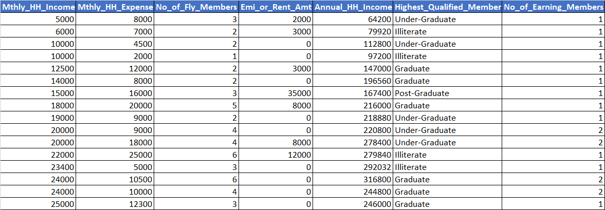
We will use the datafile inc_exp_data.csv to learn multiple linear regression in Python/R. Click here to download the file from the Resources section.

/* Import the File */

import pandas as pd
inc_exp = pd.read_csv("Inc_Exp_Data.csv")


### R code to import the File ### 
inc_exp <- read.csv("Inc_Exp_Data.csv")

View Data

inc_exp.head(16) ### Python syntax to view data

View(inc_exp)### R syntax to view data

Metadata

Hypothesis

A hypothesis is an opinion of what you expect. While framing a hypothesis, remember it should contain an independent and dependent variable. It plays a very important role in machine learning, as such, a Data Scientist should give considerate time to hypothesis development and hypothesis testing.

Herein, I am writing my hypothesis for the first 3 independent variables:

The hypothesis can be validated using graphical methods like scatter plot, numerical methods like correlation analysis and regression. We will test our hypothesis using:

• Scatter plots (pair plots)
• P-value of the independent variables in the Linear Regression model

Pair Plots

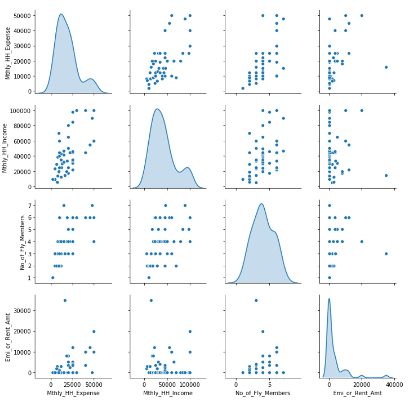
It is a good practice to perform univariate and bivariate analyses of the data before building the models. Pair Plots are a really simple (one-line-of-code simple!) way to visualize relationships between each variable.

# Import the seaborn package for visualization 
import seaborn as sns
%matplotlib inline 
sns.pairplot(inc_exp[ ['Mthly_HH_Expense', 'Mthly_HH_Income', 
    'No_of_Fly_Members', 'Emi_or_Rent_Amt'] ], 
    diag_kind = 'kde')

# Import Data
inc_exp <- read.csv("Inc_Exp_Data.csv")

# View Data
View(inc_exp)

# Pair Plots
# install.packages("psych") 
library(psych)
pairs.panels(
  inc_exp[1:4], 
  method = "pearson", # correlation method
  hist.col = "#00AFBB",
  density = TRUE, # show density plots
  lm = TRUE # plot the linear fit
)

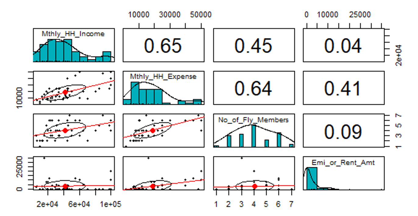
Inferences from Pair Plots:

1. The trends between the dependent and independent variables are as per our hypothesis.
2. The distribution of the Mthly_HH_Expense, Mthly_HH_Income, and No_of_Fly_Members variables is some-what Normal Distribution.
3. The Emi_or_Rent_Amt is highly skewed. Many observations have value as 0.

Build the Model

## Multiple Linear Regression 

import statsmodels.formula.api as sma 

m_linear_mod = sma.ols( formula = "Mthly_HH_Expense ~ Mthly_HH_Income 
    + No_of_Fly_Members + Emi_or_Rent_Amt", 
    data = inc_exp).fit() 

m_linear_mod.summary()

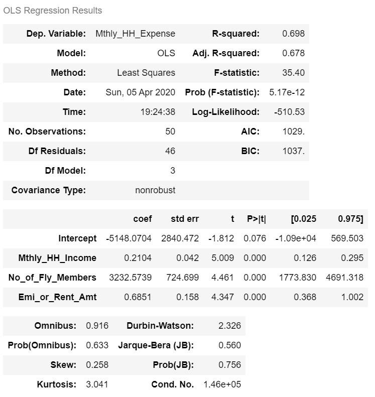
 # Build the Model

m_linear_mod <- lm( Mthly_HH_Expense ~ Mthly_HH_Income 
                    + No_of_Fly_Members + Emi_or_Rent_Amt, 
                    data = inc_exp ) 

summary(m_linear_mod)

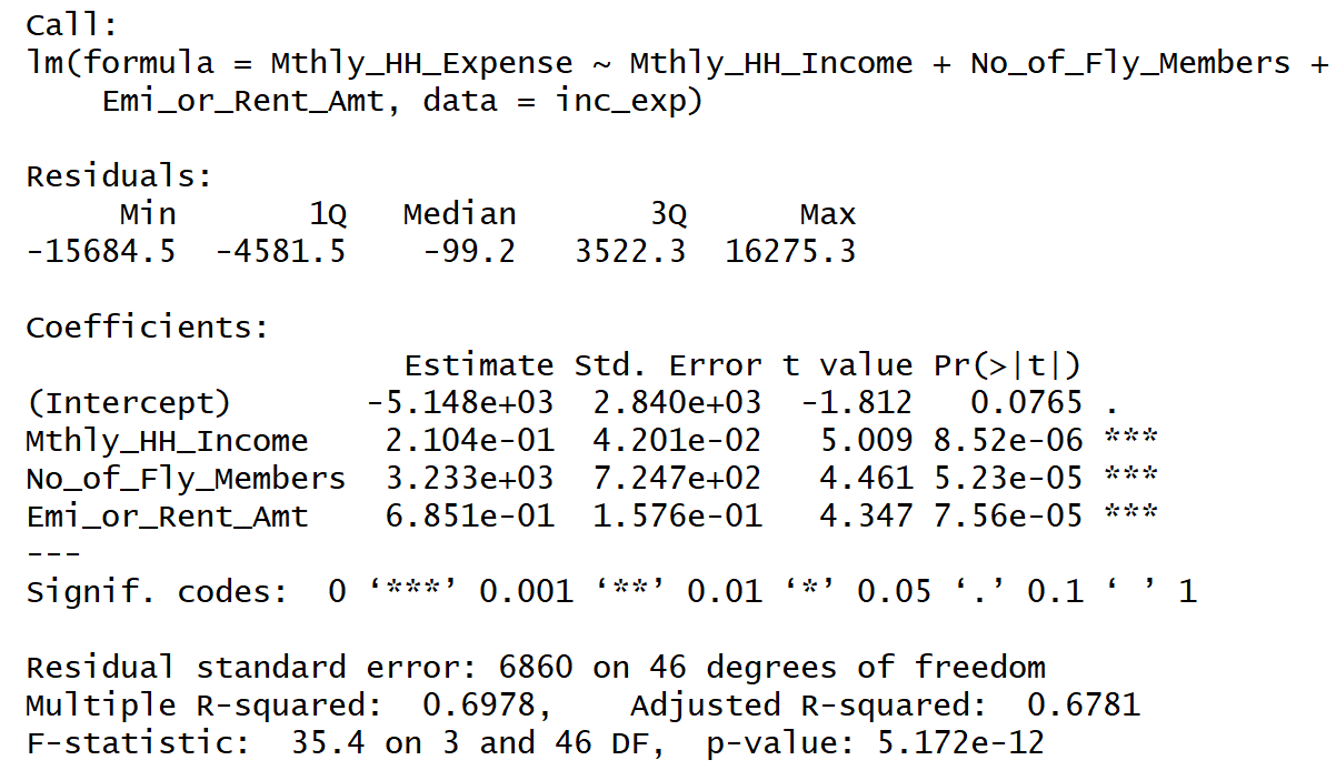
Interpretation of Regression Summary:

1. Adjusted R-squared of the model is 0.6781. This statistic has to be read as “67.81% of the variance in the dependent variable is explained by the model”.

2. All the explanatory variables are statistically significant. (p-values < alpha; assume alpha = 0.0001).

3. The beta coefficient sign (+ or -) are in sync with the correlation trends observed between the dependent and the independent variables.

4. The p-value of the F Test statistic is 5.7e-12. We conclude that our linear regression model fits the data better than the model with no independent variables.

Adjusted R-squared

Adjusted R Squared as the term suggests is R Squared with some adjustment factor. The Adjusted R Squared is a modified version of R Squared that has been adjusted for the number of predictor variables in the model.

Why use Adjusted R-Squared and not R-Squared?

Assume, you have a random variable having a casual relationship with the dependent variable. The addition of such a random variable to the model will still improve the model’s R-squared statistic. However, the Adjusted R Squared statistic will decrease and penalize the model if the explanatory variable does not contribute to the model. It is evident from the Adjusted R-Squared formula.

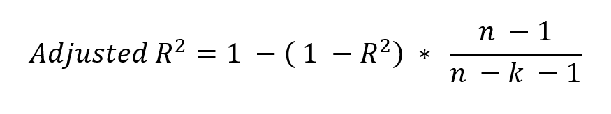
Where n is No. of Records and k is No. of Variables.
The denominator (n – k – 1) penalizes the R² for every additional variable. If the added variable does not improve the Model R², then the Adjusted R² value will decrease. The drop in Adjusted R² suggests the added term should be dropped from the model.

Let us understand Adjusted R-Squared with practical example

Let us add a Sr_No column to the data and use it as an explanatory variable.

## Multiple Linear Regression 

import statsmodels.formula.api as sma 

m_linear_mod = sma.ols( formula = "Mthly_HH_Expense ~ Mthly_HH_Income 
    + No_of_Fly_Members + Emi_or_Rent_Amt + Sr_No", 
    data = inc_exp).fit() 


print("The model R-Squared is", m_linear_mod.rsquared.round(4))
print("The model Adj. R-Squared is", m_linear_mod.rsquared_adj.round(4))

The model R-Squared is 0.7022
The model Adj. R-Squared is 0.6757

m_linear_mod <- lm( Mthly_HH_Expense ~ Mthly_HH_Income 
                    + No_of_Fly_Members + Emi_or_Rent_Amt + Sr_No, 
                    data = inc_exp ) 

model_summary = summary(m_linear_mod)

cat("The model R-Squared is", model_summary$r.squared)
cat("The model Adj. R-Squared is", model_summary$adj.r.squared)

The model R-Squared is 0.7022044
The model Adj. R-Squared is 0.6757337

Interpretation

By adding Sr_No term, the R-Squared has increased from 0.6978 to 0.7022. However, Adjusted R-Squared has decreased from 0.6781 to 0.6757. As Adjusted R-Squared has decreased, the added term (Sr_No) should be dropped from the model.

Next Blog

In our upcoming blog, we will explain the concept of Multicollinearity, Prediction using the model, and more.

<<< previous blog          |         next blog >>>
Linear Regression blog series home