Simple Linear Regression is a linear regression with only one explanatory variable. In this blog, we will learn to build a simple linear regression model in Python and R along with a detailed explanation of the model summary output. We will use the datafile inc_exp_data.csv to build the model. Click here to download the file from our Resources section.

I hope you would have downloaded the file. Let’s get started !!!

Simple Linear Regression Model Development

Import Data

### Python code to import the File ###

import pandas as pd

inc_exp = pd.read_csv("Inc_Exp_Data.csv")


### R code to import the File ###

inc_exp <- read.csv("Inc_Exp_Data.csv")

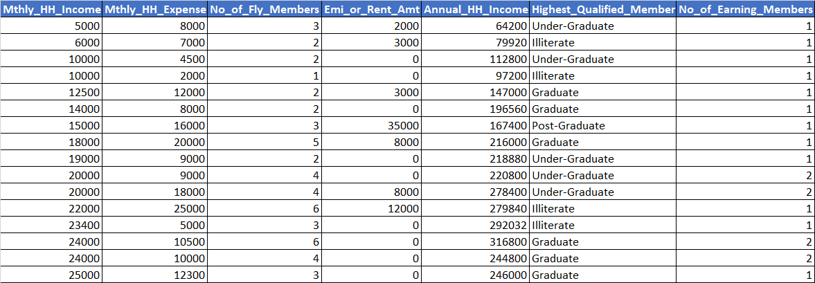
View Data

inc_exp.head(16) ### Python syntax to view data

View(inc_exp)    ### R syntax to view data

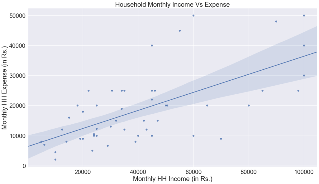
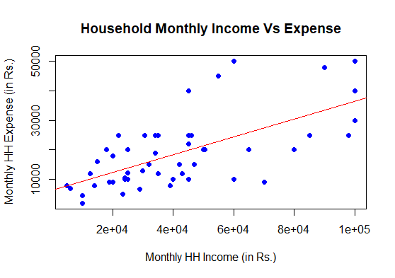
Scatter Plot

Scatter plots are a great way to check linearity between two variables. It is a recommended practice to visually check the linearity between the dependent & independent variables before running regression code for model development.

# Scatter Plot in Python

import seaborn as sns
sns.regplot(inc_exp['Mthly_HH_Income'], 
     inc_exp['Mthly_HH_Expense']).set(
     title = 'Household Monthly Income Vs Expense',
     xlabel = 'Monthly HH Income (in Rs.)', 
     ylabel = 'Monthly HH Expense (in Rs.)' 
)

# Scatter plot in R

plot ( x = inc_exp$Mthly_HH_Income, 
       y = inc_exp$Mthly_HH_Expense,    
       main = "Household Monthly Income Vs Expense",    
       xlab = "Monthly HH Income (in Rs.)",
       ylab = "Monthly HH Expense (in Rs.)",
       pch = 19, col = "blue" )


abline( lm(Mthly_HH_Expense ~ Mthly_HH_Income, 
        data = inc_exp), 
       col= "red" )

Correlation Check

#Correlation Coefficient in Python

import numpy as np
cor = np.corrcoef(inc_exp['Mthly_HH_Income'], 
     inc_exp['Mthly_HH_Expense'])
cor[1,0]

Out[6]: 0.6492152549316462



#Correlation Coefficient in R

cor = cor(inc_exp$Mthly_HH_Income, inc_exp$Mthly_HH_Expense)
cor
[1] 0.6492153

From the correlation coefficient value, we can infer that there is a reasonably good correlation between the Income and Expense variable.

Build the Model

/* Build the linear model */

import statsmodels.api as sm
xdat = inc_exp['Mthly_HH_Income']
xdat = sm.add_constant(xdat)
ydat = inc_exp['Mthly_HH_Expense']
model = sm.OLS(ydat, xdat).fit()
model.summary()

linear_mod <- lm( 
     formula = Mthly_HH_Expense ~ Mthly_HH_Income, 
     data = inc_exp 
)

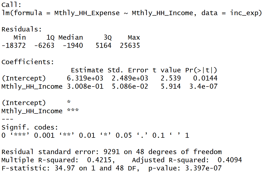
Interpretation of Model Summary Output

1. Check the p-value of the independent variable

Null Hypothesis – In regression, the null hypothesis is that the beta coefficient of all independent variables is 0, i.e., the dependent variable is not a function of an independent variable.
For more clarity, I am stating the same in different words as, the dependent variable (Monthly Household Expense in above e.g.) is not dependent on the explanatory variable (Monthly Household Income)

Alternate Hypothesis – the beta coefficient of at least one of the independent variables is not 0, i.e., there is at least one explanatory variable with a non-zero beta coefficient.
For more clarity, I am stating the same in different words as, the dependent variable (Monthly Household Expense in above e.g.) is dependent on the explanatory variable (Monthly Household Income)

Assuming the alpha threshold of 0.05
The p-value from the above summary is 0.000, which means, we may reject the null and accept the alternate hypothesis. That is, the Monthly Household Income is a significant variable.

Whenever we build a regression model, we should ensure the p-value of all independent variables should be less than the alpha-threshold.

2. Check the beta coefficient sign (+ or -)

From the scatter plot we observe that there is a positive correlation between the dependent and independent variables. As such, the beta estimate of the independent variable should also be positive.
The beta estimate of the Income variable is +0.3008. The sign of the beta coefficient is in sync with the correlation trend between Income & Expense.

3. Linear Equation

From summary we observe:
Intercept = 6319.10
Mthly_HH_Income (Beta Estimate) = 0.3008

The linear equation will be:
Monthly Expense = 6319.10 + 0.3008 * Monthly Income

If the Monthly Income of a household is 0, then the household’s estimated monthly expense is Rs. 6319/-.
If the Monthly Income of a household is Rs. 10000, then the expected monthly expense of the household is Rs. 9327.10/- (= 6319.10 + 0.3008 * 10000).

4. R-Squared

R–squared is a statistical measure of how close the data are to the fitted regression line. It is also known as the Coefficient of Determination. The  R-Squared value of our simple linear regression model is 0.421. It signifies that 42.1% of the variance in the dependent variable (Mthly_HH_Expense) is explained by the independent variable (Mthly_HH_Income). Typically, for a good linear model, we should have an R Squared value of 0.8 and above.

Let’s proceed to R Squared, Adjusted R Square, Multiple Linear Regression, and other concepts of the Linear Regression.

Thank you.

<<< previous blog          |         next blog >>>
Linear Regression blog series home

Related Read: Data Science Certification Program