Measures of Relationship
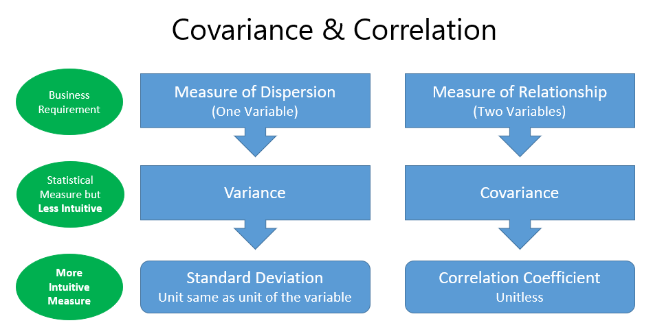
Definition: The statistical measures which show a relationship between two or more variables are called Measures of Relationship. Correlation and Regression are commonly used measures of relationship. In this blog, we will understand the Covariance measure and its calculations steps. Part 2 of this blog will explain the calculation of Correlation.
(Related read: Linear Regression Blog Series)
Covariance
Covariance is the measure of the joint variability of two random variables (X, Y). For Example – Income and Expense of Households. The households having higher Income (say X) will have relatively higher Expenses (say Y) and vice-versa. This kind of relationship between two variables is called joint variability and is measured through Covariance and Correlation.
Covariance is represented as Cov(X, Y). (Wikipedia link). The covariance can Positive, Negative, or Zero.
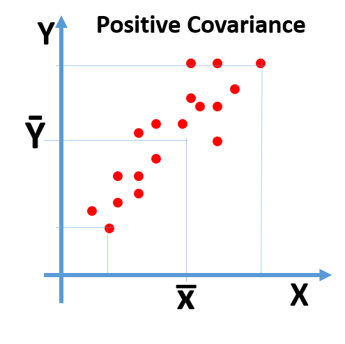
| Positive Covariance: If the variable(X) takes a higher value, the value of the corresponding variable(Y) is also higher and vice-versa.
E.x. Income and Expense of Household. As X takes a higher value, the corresponding values of Y is on the higher side |
 |
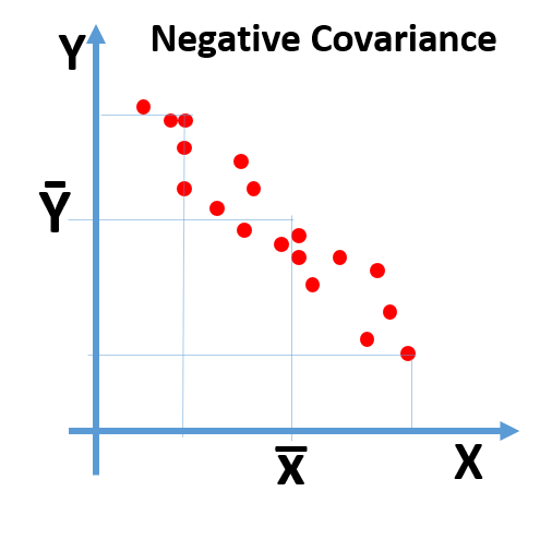
| Negative Covariance: If the variable(X) takes a higher value, the value of the corresponding variable(Y) is low and vice-versa.
Example: Price and Demand. As the Price of a commodity increases, its Demand decreases. |
 |
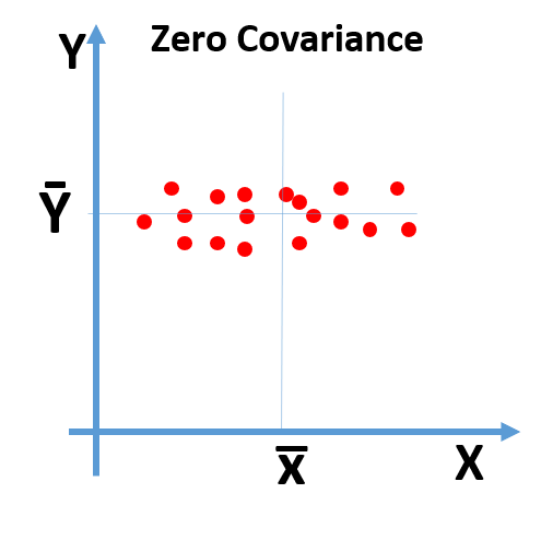
| Zero Covariance or No Covariance: There is no linear relationship between variable(X) and variable(Y).
Note: The Zero Covariance means the covariance will be zero or near zero |
 |
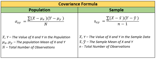
Formula
Hands-on Example
To understand the concept of covariance, it is important to do some hands-on activity. A sample survey data of 15 households is given below. The fields are Monthly Income, Monthly Expense, and Annual Income details of the households.
| Mthly_HH_Income | Mthly_HH_Expense | Annual_HH_Income |
| 5000 | 8000 | 64200 |
| 6000 | 7000 | 79920 |
| 10000 | 4500 | 112800 |
| 10000 | 2000 | 97200 |
| 12500 | 12000 | 147000 |
| 14000 | 8000 | 196560 |
| 15000 | 16000 | 167400 |
| 18000 | 20000 | 216000 |
| 19000 | 9000 | 218880 |
| 20000 | 9000 | 220800 |
| 20000 | 18000 | 278400 |
| 22000 | 25000 | 279840 |
| 23400 | 5000 | 292032 |
| 24000 | 10500 | 316800 |
| 24000 | 10000 | 244800 |
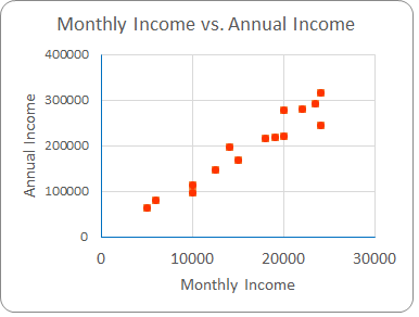
Scatter Plot
A scatter plot is best used to visually see the linear relationship between X and Y.
 |
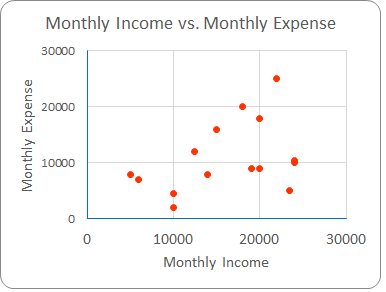 |
| From the above two scatter plots we can see that Monthly Income has positive covariance with both the variables, Annual Income, and Monthly Expense.
However, the linearity between Monthly Income and Annual Income appears to be much strong as compared to the relationship between Monthly Income and Monthly Expense. The strength of the linear relationship between two continuous variables is measured by a statistical measure called Correlation |
|
Covariance Calculations
Let us denote Monthly Household Income as X and Monthly Household Expense as Y. Then the covariance of Monthly Income and Expense is:
Cov(X,Y) = sum( (X - mean(x)) * (Y - mean(y)) ) / (n - 1)
Mean calculation
# Calculating mean(X)
mean(x) = (5000+6000+10000+10000+12500+14000+15000+18000+19000+20000+20000+22000+23400+24000+24000) / 15
mean(x) = 242900 / 15
mean(x) = 16193.33

# Calculating mean(Y)
mean(y) = (8000+7000+4500+2000+12000+8000+16000+20000+9000+9000+18000+25000+5000+10500+10000) / 15
mean(y) = 164000 / 15
mean(y) = 10933.33
Intermediate covariance calculation steps
|
Monthly Inc. |
Monthly Exp. (Y) |
X – mean(x) | Y – mean(y) | (X – mean(x)) * (Y – mean(y)) |
| 5000 | 8000 | -11193.33 | -2933.33 | 32833777.78 |
| 6000 | 7000 | -10193.33 | -3933.33 | 40093777.78 |
| 10000 | 4500 | -6193.33 | -6433.33 | 39843777.78 |
| 10000 | 2000 | -6193.33 | -8933.33 | 55327111.11 |
| 12500 | 12000 | -3693.33 | 1066.67 | -3939555.56 |
| 14000 | 8000 | -2193.33 | -2933.33 | 6433777.78 |
| 15000 | 16000 | -1193.33 | 5066.67 | -6046222.22 |
| 18000 | 20000 | 1806.67 | 9066.67 | 16380444.44 |
| 19000 | 9000 | 2806.67 | -1933.33 | -5426222.22 |
| 20000 | 9000 | 3806.67 | -1933.33 | -7359555.56 |
| 20000 | 18000 | 3806.67 | 7066.67 | 26900444.44 |
| 22000 | 25000 | 5806.67 | 14066.67 | 81680444.44 |
| 23400 | 5000 | 7206.67 | -5933.33 | -42759555.56 |
| 24000 | 10500 | 7806.67 | -433.33 | -3382888.89 |
| 24000 | 10000 | 7806.67 | -933.33 | -7286222.22 |
|
Sum(X – mean(x)) * (Y – mean(y)) |
223293333.33 | |||
Final covariance calculation step
n = 15
mean(x) = 16193.33
mean(y) = 10933.33
sum( (X - mean(x)) * (Y - mean(y)) ) = 223293333.33

#Therefore the Covariance of Sample monthly Household Income and Expence is
Cov(X,Y) = sum( (X - mean(x)) * (Y - mean(y)) ) / (n - 1)
Cov(X,Y) = 223293333.33 / (15 - 1) => 223293333.33 / 14
Cov(X,Y) = 15949523.81


Cov(Monthly Income , Monthly Expense) = 15949523.81
Interpretation of Covariance
- The covariance between the Monthly Income and the Monthly Expense is 15949523.81.
- It is a positive number, hence we conclude there is a positive relationship between Monthly Household Income and the Expense. i.e., when the Monthly Household Income takes a higher value, the corresponding Expense value is also likely to be higher and vice-versa.
Disadvantage of Covariance
- Covariance only measures the direction of the relationship, but it does not measure the strength of the relationship. In order to measure the strength, we need to calculate the normalized version of covariance, i.e., Correlation
Application of Variance-Covariance: Beta of Stock
The variance-covariance measures do not have any business meaning by themselves. However, these measures are used in calculations of other test statistics like ANOVA, R-Squared, hypothesis testing, statistical inference, and more. One practical application of Variance-Covariance is in calculating the Beta of Stock. Beta is a concept that measures the expected move in a stock relative to movements in the overall market. (Investopedia article on Beta of Stock)
Correlation
- Covariance only shows the direction of the linear relationship between two Variables (I.e., Positive, Negative, or No Covariance). It cannot measure the strength of the relationship between the two variables.
- To measure both the strength and direction of the linear relationship between two variables, we use a statistical measure called correlation.
- The correlation only measures the association. The Association is not Causation.
Formula
- The Formula to Calculate the Correlation Coefficient (r) between Variable is
r = Covariance(x,y) / ((Standard deviation of X) * (Standard deviation of Y))
- ‘r’ takes any value between -1 and 1
Correlation Range Interpretation r = 1 Perfectly Positive Linear Relationship between two variables r = -1 Perfectly Negative Linear Relationship between two variables r = 0 No Relationship between two variables
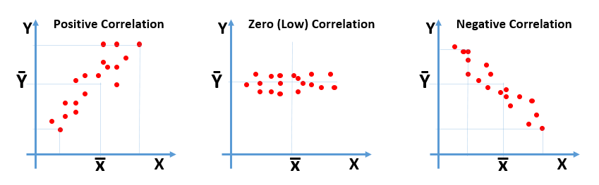
Positive, Negative, Zero Correlations
The two variables(X, Y) can have Positively Correlation, Negatively Correlation, or Zero correlation.
| Correlation | Description |
| Positive Correlation
|
|
| Negative Correlation
|
|
| No Correlation
|
|
Hands-on Example
Let’s calculate the correlation coefficient between two variables (monthly Income, Monthly Expense) for 15 sample household Survey data given in the below table.
| Mthly_HH_Income | Mthly_HH_Expense | Annual_HH_Income |
| 5000 | 8000 | 64200 |
| 6000 | 7000 | 79920 |
| 10000 | 4500 | 112800 |
| 10000 | 2000 | 97200 |
| 12500 | 12000 | 147000 |
| 14000 | 8000 | 196560 |
| 15000 | 16000 | 167400 |
| 18000 | 20000 | 216000 |
| 19000 | 9000 | 218880 |
| 20000 | 9000 | 220800 |
| 20000 | 18000 | 278400 |
| 22000 | 25000 | 279840 |
| 23400 | 5000 | 292032 |
| 24000 | 10500 | 316800 |
| 24000 | 10000 | 244800 |
Correlation Calculations
- Let X be the Monthly Income and Y be Monthly Expense, Then the Correlation coefficient r is,
r = Cov(X,Y) / (Std(X) * Std(Y))
- In the previous blog, We have already calculated the Covariance between the Variable Monthly Income and Monthly Expense. Refer to the Previous blog for Covariance calculations.
Cov(X,Y) = 15949523.81
- Mean Calculations
#Calculating mean(X)
mean(x) = (5000+6000+10000+10000+12500+14000+15000+18000+19000+20000+20000+22000+23400+24000+24000) / 15
mean(x) = 242900 / 15
mean(x) = 16193.33
#Calculating mean(Y)
mean(y) = (8000+7000+4500+2000+12000+8000+16000+20000+9000+9000+18000+25000+5000+10500+10000) / 15
mean(y) = 164000 / 15
mean(y) = 10933.33
- Intermediate Correlation Calculations
Mthly_HH_Income (X) Mthly_HH_Expense (Y) X – Mean(X) (X – Mean(X))^2 Y – Mean(Y) (Y – Mean(Y))^2 5000.00 8000.00 -11193.33 125290711.11 -2933.33 8604444.44 6000.00 7000.00 -10193.33 103904044.44 -3933.33 15471111.11 10000.00 4500.00 -6193.33 38357377.78 -6433.33 41387777.78 10000.00 2000.00 -6193.33 38357377.78 -8933.33 79804444.44 12500.00 12000.00 -3693.33 13640711.11 1066.67 1137777.78 14000.00 8000.00 -2193.33 4810711.11 -2933.33 8604444.44 15000.00 16000.00 -1193.33 1424044.44 5066.67 25671111.11 18000.00 20000.00 1806.67 3264044.44 9066.67 82204444.44 19000.00 9000.00 2806.67 7877377.78 -1933.33 3737777.78 20000.00 9000.00 3806.67 14490711.11 -1933.33 3737777.78 20000.00 18000.00 3806.67 14490711.11 7066.67 49937777.78 22000.00 25000.00 5806.67 33717377.78 14066.67 197871111.11 23400.00 5000.00 7206.67 51936044.44 -5933.33 35204444.44 24000.00 10500.00 7806.67 60944044.44 -433.33 187777.78 24000.00 10000.00 7806.67 60944044.44 -933.33 871111.11 sum((X – mean(X))^2) 573449333.33 sum((Y – mean(Y))^2) 554433333.33
- Standard deviation Calculations
Total Number of Observation, n = 15

#Standard deviation of X
Std(X) = sqrt(sum((X - mean(X))^2) / (n - 1))
sum((X - mean(X))^2)= 573449333.33 #From the Above table
Std(X) = sqrt((573449333.33) / (15 - 1)) => sqrt((573449333.33) / (14))
Std(X) = sqrt(40960666.67)
Std(X) = 6400.05

#Standard deviation of Y
Std(Y) = sqrt(sum((Y - mean(Y))^2) / (n - 1))
sum((Y - mean(Y))^2)= 554433333.33 #From the Above table
Std(Y) = sqrt((554433333.33) / (15 - 1)) => sqrt((554433333.33) / (14))
Std(Y) = sqrt(39602380.95)
Std(Y) = 6293.04
- Final Correlation Calculation
Cov(X,Y) = 15949523.81
Std(X) = 6400.05
Std(Y) = 6293.04

#Correlation Coefficient
r = Cov(X,Y) / (Std(X) * Std(Y))
r = 15949523.81 / (6400.05 * 6293.04)
r = 15949523.81 / 40275770.65
r = 0.396
The correlation between monthly Income and monthly Expense is 0.396. Therefore, there is a Low Positive correlation between Monthly Household Income (X), and the Monthly Household Expense (Y).
Practice Exercise
- Calculate the Correlation coefficient between Monthly Household Income and Annual Household Income for data that we used as an example and complete the following Table.
- Total Number of Observations (n)
- Mean of Monthly Household Income
- Mean of Annual Household Income
- The covariance of Monthly Household Income and Annual Household Income
- The Standard Deviation of Monthly Household Income
- The Standard Deviation of Annual Household Income
- The Correlation Coefficient r
- Is the linear relationship between the two variable is positive or negative and Explain it?
Next Blog
- We will discuss the Answers to our Practise Exercises. Later, We will discuss the Graphical Methods in Descriptive Statistics.