K Means Clustering in R

Why Clustering?

Clustering is done to group similar objects/entities.
To create homogeneous groups from heterogeneous data.
E.g. in Marketing, we create Customer Segments (Clusters) to design customized products/services/offerings at the segment level.

What is Clustering?

Clustering is Machine Learning and technical approach of doing Segmentation.
Clustering is a Machine Learning Technique for finding similar groups in data, called “clusters”

What is a Cluster?

A cluster can be defined as a collection of objects which are “similar” between them and are “dissimilar” to the objects belonging to other clusters

Broad Types of Clustering

Hierarchical Clustering
Partitioning Clustering

Code to Perform K Means Clustering in R

Setting the Working Directory:

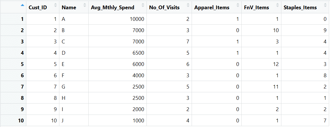
The data file we will use is “Cust_Spend_Data.csv” and it can be downloaded from the Complementary Resources section on our website. After having downloaded the file, say the file is saved in the folder “D:/K2Analytics/datafile”

> setwd ("D:/K2Analytics/datafile")

Import Data:

> KRCDF <- read.csv("Cust_Spend_Data.csv", header=TRUE)

View Data:

> View(KRCDF)

Understand Data:

The data is about Retail Customer Spends at Supermarket. The column metadata is:

AVG_Mthly_Spend: The average monthly amount spent by the customer
No_of_Visits: The number of times a customer visited the Supermarket in a month
Item Counts: Count of Apparel, Fruits and Vegetable (FnV), Staple Items purchased in a month

Scale Data:

In clustering, if the data is not ordinal then we should scale the data. To scale we can use scale() function in R which standardizes the data.

> scaled.KRCDF <- scale(KRCDF[,3:7])

Optimal Number of Clusters:

Identifying the optimal number of clusters using SCREE Plot of Within-Sum-of-Squares (WSS).

## code taken from the R-statistics blog
> wssplot <- function(data, nc=15, seed=1234){
   wss <- (nrow(data)-1)*sum(apply(data,2,var))
   for (i in 2:nc){
set.seed(seed)
   wss[i] <- sum(kmeans(data, centers=i)$withinss)
   }
plot(1:nc, wss, type="b", xlab="Number of Clusters",
ylab="Within groups sum of squares")
}
> wssplot(scaled.KRCDF, nc=5)

The output of wssplot function is SCREE Plot

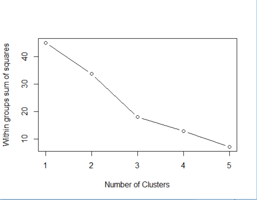
In the Scree Plot we have to see the point of “Elbow Formation”.
The elbow point is the optimal number of clusters. From the plot, I guess that the elbow formation is at N = 3

Another approach to finding an optimal number of clusters in R is using NbClust package. The documentation of NbClust packages reads- “NbClust package provides 30 indices for determining the number of clusters and proposes to a user the best clustering scheme from the different results obtained by varying all combinations of several clusters, distance measures, and clustering methods.”

## install.packages("NbClust")
> library(NbClust)
> ?NbClust
> nc <- NbClust(KRCDF[,c(-1,-2)], min.nc=2,
max.nc=4, method="kmeans")

The output of the NbClust function suggests that 3 is the optimal number of clusters.

Run K Means Clustering

> kmeans.clus = kmeans(x=scaled.KRCDF, centers = 3)

centers = 3 parameter is to suggest the number of clusters you want

Creating cluster label in our original dataset

> KRCDF$Clusters <- kmeans.clus$cluster

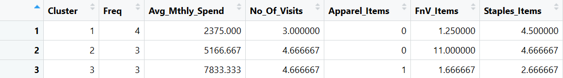
Profiling the Clusters

Let us profile the clusters to understand their characteristics. It involves aggregating and summarizing data at the cluster level.

> aggr = aggregate(KRCDF[,-c(1,2,8)],
list(KRCDF$Clusters), mean)

> clus.profile <- data.frame( Cluster=aggr[,1],
Freq=as.vector(table(RCDF$Clusters)), aggr[,-1] )

> View(clus.profile)

Validating the Clusters

This step is to understand the characteristics of the clusters. See if the clusters make business sense and how it can be used for Marketing or the purpose for which clustering exercise is undertaken.

From profiling we see:

Cluster 1 – Low Spend, Low Visit Frequency, and they majorly buy staple items.
Cluster 2 – Moderate Avg. Monthly Spend. They come at least 4 – 5 times in a month to buy regular household items.
Cluster 3 – Highest Avg. Monthly Spend. These customers 4 to 5 times in a month and have shopped in Apparel Section.

The clusters have differentiating characteristics that enables a marketer to design suitable offers and campaigns for them.

Visually representing the Clusters

A visual depiction of the clusters helps us see how dis-similar or apart the clusters are from each other

> library(cluster)
> clusplot(scaled.KRCDF, kmeans.clus$cluster,
color=TRUE, shade=TRUE, labels=2, lines=1)

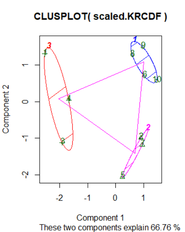
Component 1 and Component 2 in the above Cluster Plot are the Principal Components.

From the plot, we can infer that the three clusters are dissimilar from each other.

Naming the Clusters

In the end, we must give self-explanatory names to clusters. The cluster names will help in relating to the clusters. E.g. we may call Cluster 1 as Apparel Buyers, Cluster 2 as FnV Lovers, and Cluster 3 as Low-Low Segment.

Sign-Off Note: I hope you enjoyed doing K Means Clustering using R!

Suggested read – Hierarchical Clustering using R

Connect with us on our Official Data Science Mumbai, Meetup Community